
CHAPTER 2 · FMC / TFM / PCI Level 2
UT Level 2 Foundations for Advanced Imaging
In this chapter · 14 sections
Learning outcomes
After completing this chapter, the learner should be able to:
relate velocity, frequency and wavelength to ultrasonic behaviour and image resolution;
apply the declared angle convention when using Snell's law;
calculate pulse-echo and pitch-catch travel times for simple paths;
distinguish RF amplitude, polarity, phase, envelope and time position;
use decibels correctly and recognise their amplitude-domain limitation;
relate sampling interval and bandwidth to the recorded waveform;
explain axial, lateral and orientation-dependent resolution; and
recognise foundation errors that will propagate into FMC, TFM and PCI.
Crossover map
| UT Level 2 foundation | Why it matters in FMC/TFM/PCI | Failure if neglected |
|---|---|---|
| Velocity and time of flight | Reconstruction delays depend on the travel-time model | Responses defocus, move or split |
| Wavelength and bandwidth | Control interaction and achievable resolution | Pixel size is mistaken for physical resolution |
| Snell's law and mode conversion | Define valid paths through interfaces | Wrong mode or angle is reconstructed |
| RF phase and polarity | TFM reinforcement and PCI depend on waveform behaviour | Envelope-only thinking hides phase errors |
| dB and dynamic range | Still govern amplitude setup and data quality | Coherence is incorrectly treated as amplitude |
| Reflector orientation | Controls returned energy and diffraction | Image shape is mistaken for flaw shape |
| Coupling and attenuation | Determine whether useful pair data exist | Processing is expected to recover absent information |
Velocity, frequency and wavelength
Wave velocity is primarily a property of the material and propagation mode. Frequency describes cycles per second. Wavelength is the distance occupied by one cycle in the material. For a declared mode velocity V in metres per second and frequency f in hertz, wavelength lambda is:
lambda_m = c_m / f
If shear-wave velocity in steel is taken as 3,250 m/s and frequency is 5 MHz, the wavelength is approximately 0.65 mm. The value is not a universal resolution claim. A reflector must still scatter energy back toward the usable aperture, and the complete pulse bandwidth, aperture, geometry and signal-to-noise ratio affect what can be separated.
Higher frequency generally reduces wavelength and can improve spatial discrimination, but it commonly increases attenuation and sensitivity to surface condition, grain structure and coupling. Lower frequency can improve penetration while producing a longer pulse and broader response. Probe selection is therefore a trade-off tied to the examination objective, not a competition for the largest number printed on a data sheet.
Bandwidth describes the useful frequency range within a pulse. A broad-band pulse can be shorter in time, supporting improved axial separation, but may have lower peak response or different penetration behaviour. Reconstruction and phase processing also depend on the recorded frequency content. Filters that remove useful bandwidth can change response form, timing and phase.
Refraction and mode conversion
At an interface, the incident wave can reflect and transmit as one or more modes. The relationship between wave angles and velocities is expressed by Snell's law. In this manual, angles are measured from the surface normal unless a figure explicitly states otherwise.
sin(theta_1) / c_1 = sin(theta_2) / c_2
For an incident wave in a wedge, the transmitted longitudinal and shear modes in the component can have different angles because their velocities differ. At particular incident angles a transmitted mode approaches 90 degrees from the normal and no longer propagates into the second material as a bulk refracted wave. These critical-angle concepts matter when selecting a wedge and when checking whether a proposed TFM path is physically available.
Snell's law is not merely a setup calculation. TFM predicts travel time through wedge and component legs. If the wrong velocity, interface position or mode is selected, calculated rays arrive at the wrong pixel or do not align across the aperture. A phase-coherence image can be particularly sensitive to timing-model error because phase agreement is reduced when the predicted sample positions are wrong.
The simple flat-interface model assumes isotropic, homogeneous materials. Austenitic weld metal, composites, coarse-grained material, cladding, curvature and temperature gradients can produce direction-dependent velocity, beam distortion and scattering. A technician should not force a simple model onto a component merely because the software permits it.
Time of flight and pair geometry
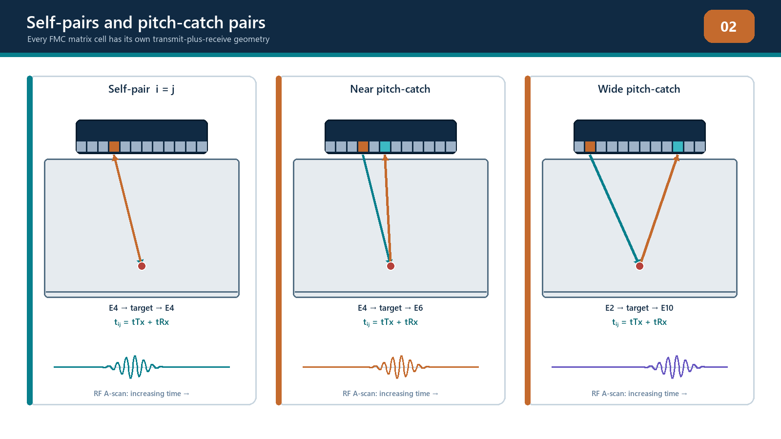
For a conventional pulse-echo path in one homogeneous mode, total time is twice the one-way distance divided by velocity. An FMC off-diagonal pair is pitch-catch: the transmitter and receiver occupy different positions, so total time is the transmit-leg time plus the receive-leg time. The path lengths are generally different and must be calculated from the declared geometry.
Consider a point P at depth z below an array. If transmitter i and receiver j are at horizontal coordinates xi and xj, the direct homogeneous distances are:
transmit distance: the straight-line distance from (xi,0) to (xP,zP);
receive distance: the straight-line distance from (xP,zP) to (xj,0); and
total time: (transmit distance + receive distance) / V.
This pair-specific time is the foundation of direct-mode TFM. Wedges, refracting interfaces, skips and mode conversion add further path legs and velocities. A depth conversion based on a single two-way pulse-echo path cannot simply be applied to every matrix cell.
Sampling and the recorded waveform
The instrument records a continuous electrical signal at discrete time intervals. If sampling frequency is fs, the sample period Ts is:
Delta t = 1 / f_s
For example, 100 MHz sampling produces a nominal interval of 10 ns. At shear velocity 3,250 m/s, that interval corresponds to 0.0325 mm of one-way travel in a homogeneous material. It does not mean the system can resolve features separated by 0.0325 mm. It only describes time sampling. Pulse length, bandwidth, aperture, noise and reconstruction determine physical resolution.
The acquisition start, electronic delay, wedge delay and pre-trigger must be distinguished. Sample index zero is not automatically the component surface. Metadata must preserve the sampling frequency, sample count, time origin, filters and signal representation. Without them, a set of numbers cannot be placed reliably in time or space.
Sampling must be sufficient for the retained frequency content. Inadequate sampling can distort frequency and phase, while excessive sampling increases data volume without creating new acoustic bandwidth. Timing jitter or inconsistent channel delay can reduce TFM reinforcement and phase coherence even when individual A-scans appear plausible.
RF amplitude, polarity, phase and envelope
An RF A-scan is bipolar: voltage moves positive and negative around a baseline. Amplitude describes magnitude. Polarity identifies sign at a given instant. Phase identifies position within a waveform cycle or frequency component. Envelope is a positive magnitude representation surrounding the oscillating RF packet.
Envelope displays are useful for conventional amplitude measurement and make response packets easy to see. They hide the sign changes needed to understand constructive and destructive summation. If several pair traces are sampled at the correct travel time and the same phase feature aligns, their signed values reinforce. If a wrong pixel or model samples mixed positive and negative lobes, the sum can cancel.
PCI uses phase-related information rather than conventional amplitude summation, but that does not make acquisition amplitude irrelevant. A waveform buried below electronic or material noise does not contain reliable phase evidence. A clipped waveform has lost its original form. Poor coupling can remove or destabilise data. Phase processing cannot restore information that was never recorded correctly.
Decibels and dynamic range
The decibel is a logarithmic expression of a ratio. For two compatible ultrasonic amplitudes A2 and A1, the amplitude ratio in decibels is:
Delta dB = 20 log10(A_2 / A_1)
A factor of two in amplitude corresponds to approximately 6 dB; a factor of one-half corresponds to approximately -6 dB. The sign depends on which amplitude is the numerator. Always state the reference and whether a gain change or response comparison is being described.
Dynamic range is the usable range between the smallest measurable response and the largest response that can be recorded without unacceptable distortion. Too little gain can leave useful signals near the noise floor. Too much can clip the RF waveform. TFM amplitude and PCI may respond differently to display gain or internal normalisation, but both depend on sound acquired data. A screen that refuses to look saturated does not prove the analogue-to-digital acquisition remained unclipped.
DAC, TCG and transfer correction operate in an amplitude-response framework. They may be required for a qualified amplitude-TFM technique, but they must not be transferred to amplitude-free PCI as if a coherence percentage were echo height. PCI still requires system checks, geometry calibration, performance demonstration and controlled display settings even when conventional amplitude calibration is not part of the algorithm.
Resolution, detectability and image form
Axial resolution concerns separation along the direction of propagation and is strongly influenced by pulse duration and bandwidth. Lateral resolution concerns separation across the acoustic aperture and depends on aperture, wavelength, depth, geometry and focusing. Angular discrimination concerns separation of contributions arriving from different directions. Orientation sensitivity is different: it describes how response strength and phase change as a reflector rotates relative to the insonifying and receiving apertures.
Detectability is not the same as resolution. A small isolated reflector can be detected even when its displayed spot is wider than its physical size. Two nearby reflectors can merge into one response. Conversely, a large smooth planar reflector can be poorly detected when specular energy is directed away from the array.
A TFM image shows the point-spread response of the acquisition and reconstruction system to the acoustic interaction. The apparent width or length of a bright region is not automatically the reflector dimension. Image-based sizing needs a qualified method, relevant targets and uncertainty. Pixel spacing can support coordinate reading, but it is not a certificate of measurement accuracy.
Near-surface behaviour, noise and attenuation
The initial pulse, wedge-interface response, ring-down and recovery of the receiver can obscure near-surface information. FMC includes many pair geometries, so the affected time region can vary between traces. A near-surface target may appear in some pairs or views and remain hidden in others. A demonstrated near-surface limit should be stated for each relevant path and reconstruction region.
Material attenuation reduces signal with path length and frequency. Scattering can create structured noise that sometimes aligns coherently under an incorrect or unintended path. Surface roughness and coupling variation alter transmitted and received energy. These factors should be challenged using representative specimens and multiple views, not judged from a single clean reference-block image.
Field workflow: foundation check before reconstruction
Confirm material, nominal velocities, temperature and geometry.
Declare the coordinate and angle conventions.
Verify probe frequency, bandwidth and sampling are suitable for the intended path and resolution.
Inspect representative RF A-scans before relying on processed images.
Check for clipping, low signal-to-noise ratio, unstable baseline, cross-talk and timing inconsistency.
Confirm wedge/interface delay and path timing with known reflectors.
Compare predicted and measured arrival positions.
Record any departure from the simple homogeneous model and seek approval for the method used to handle it.
Practical 2 - Predict and verify the waveform
Objective
Connect UT calculations to pair-specific FMC timing and waveform quality.
Resources
a flat homogeneous reference block with two documented targets;
an array or a supplied complete teaching dataset;
declared probe frequency and bandwidth;
declared material velocity for the selected mode; and
access to RF and envelope A-scans.
Method
Calculate wavelength at the nominal centre frequency.
Predict arrival time for one diagonal self-pair and two off-diagonal pairs for the first target.
Predict which target separation should be harder to resolve axially and explain why.
Display the matching RF traces and record measured arrival times.
Compare RF and envelope representations of the same response.
Add and remove 6 dB of amplitude gain where authorised and confirm the expected amplitude ratio without clipping.
Change only the assumed velocity in a reconstruction and observe displacement or loss of focus.
Restore the controlled setup and reverify the reference response.
Required evidence
completed calculations with units and declared assumptions;
three annotated RF traces;
a table of predicted versus measured time and difference;
one RF/envelope comparison; and
an explanation of the velocity-error effect.
Stop rules
Stop if the dataset identity, velocity, sampling frequency, time origin or pair indices are unknown. Do not adjust multiple parameters to make the prediction fit. Stop acquisition if repeated coupling or clipping prevents stable signals.
Successful completion
Predictions agree with measured values within the teaching tolerance, discrepancies are explained using physical or acquisition evidence, and the learner does not confuse sample spacing with acoustic resolution.
Common traps
Using the pulse-echo two-way depth formula for every off-diagonal pair. Each pair has separate transmit and receive legs.
Using the angle from the surface rather than from the normal. State the convention before using Snell's law.
Equating high frequency with automatically better examination. Penetration, attenuation, scattering and surface condition also change.
Reading envelope as if it preserved RF phase. It preserves magnitude information, not bipolar phase alignment.
Believing PCI can use badly clipped or noise-only data. Amplitude-free processing is not information-free processing.
Reporting a measurement to the pixel decimal place. Coordinate display precision can exceed demonstrated acoustic accuracy.
Chapter summary
TFM and PCI depend on UT foundations with less tolerance for hidden assumptions. Velocity and path geometry control predicted times. Wavelength, bandwidth and aperture control interaction and resolution. Sampling records the waveform but does not create acoustic detail. RF phase and polarity explain coherent reinforcement, while envelope and dB remain valuable amplitude-domain tools. A good crossover technician predicts timing and response behaviour before trusting the image, confirms the quality of the underlying waveforms and recognises when material or geometry invalidates the simple model.
Study and revision only. This is not an approved inspection procedure, acceptance criterion or qualification.