Artefact Diagnostics and Dataset Forensics

Why this matters

When an image looks wrong, the first useful action is usually preservation rather than adjustment. Save the original file, configuration, software identity, channel map, position data and screen evidence before changing gain, velocity, ROI or reconstruction. The first anomalous state often contains the clearest clue to root cause.

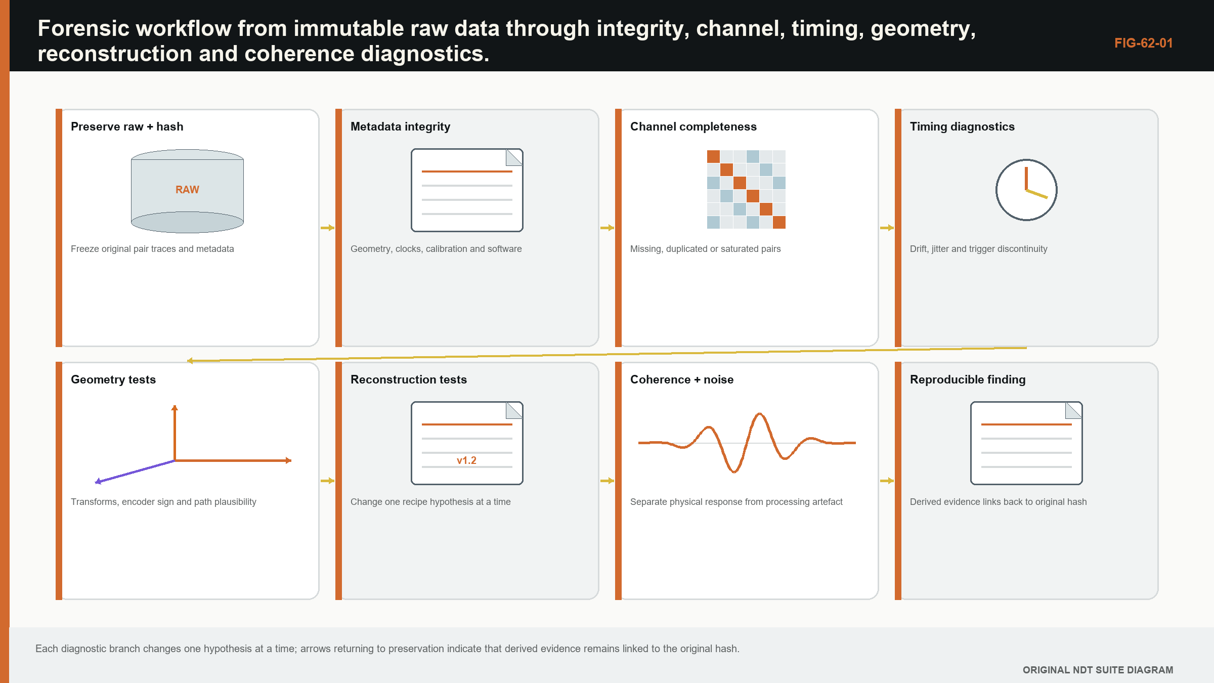
The diagnostic tree begins with three layers. First confirm file and metadata integrity. Next inspect raw traces, channel health, clipping, timing and position. Only then challenge the propagation model, reconstruction and display. Changing one controlled variable at a time turns troubleshooting into an experiment rather than a sequence of guesses.

What you already need

• Raw traces contain evidence that a final image can hide.
• Missing, clipped and zero-valued samples are not the same condition.
• Timing, position, geometry and velocity errors produce different patterns.
• A display palette can hide or exaggerate a response without changing raw data.

What you will learn

You will preserve a forensic evidence set; inspect metadata and matrix health; distinguish channel, coupling, clipping, timing, position, path and display faults; use controlled perturbations to test a suspected cause; quantify reciprocity mismatch; and record both root cause and impact on prior results.

Words you will meet

Forensics is the controlled examination of stored evidence to explain an unexpected result. Quantisation is the representation of amplitude by discrete digital levels. Registration error is a mismatch between acoustic data and its assigned position or coordinate frame. Path ambiguity occurs when more than one physical route can explain a response. A controlled perturbation is one deliberate input change used to test a diagnosis.

The Level 3 step

This chapter remains technical because the work is directly applied. The learner is not expected to diagnose every mechanism from memory. The required skill is to preserve evidence, follow a consistent tree, design a discriminating test and avoid rewriting the original state while searching for a more convenient explanation.

62.1 Preserve evidence before diagnosing

Dataset forensics begins with preservation. Copy the raw file read-only, record a cryptographic hash and retain the original directory structure, logs and setup. Reprocessing should create derived files, never overwrite the source. This protects timing, metadata and channel evidence that a quick image export would discard.

The investigation defines the symptom in measurable terms: affected positions, views, channels, time range, coordinate shift, amplitude or coherence behaviour. "The image looks wrong" is too broad. A precise symptom guides tests and prevents unrelated parameter changes.

Provenance establishes component, scan, probe, acquisition architecture, software, geometry and reconstruction recipe. Self-describing formats can store arrays and attributes, but application semantics must still be controlled. [R053] Missing provenance is itself a finding because it limits which hypotheses can be tested.

62.2 File and metadata integrity

Check file size against expected dimensions, sample type and position count. Validate headers, dataset shapes, endianness, units and checksums. A file can open while containing a truncated final position or incorrect dimension order.

Cross-check redundant metadata. Number of traces should agree with transmit and receive maps. Position count should agree with encoder arrays. Time range should agree with sample rate and sample count. Inconsistency may indicate conversion or export error.

Inspect values for impossible ranges, all-zero blocks, repeated frames and sudden scale changes. A repeated buffer can look like stable component data. Sequence numbers and timestamps help identify duplication.

62.3 Channel and coupling failures

Channel-health maps display energy, noise, saturation, delay or reciprocity residual by transmit-receive pair. A vertical stripe suggests one transmitter; a horizontal stripe suggests one receiver; a cross suggests an element involved in both roles. A checkerboard can point to multiplexing banks.

Coupling loss affects groups of channels and positions according to footprint and motion. It often reduces interface and backwall evidence together. A dead electronic channel persists regardless of coupling position. Comparing self-pairs, reciprocal pairs and neighbouring channels helps separate them.

Normalising each trace can hide weak channels. Diagnostics should begin with raw or controlled gain. Element compensation tables should be removed or accounted for when assessing hardware response.

62.4 Clipping, quantisation and dynamic range

Clipping produces flat waveform peaks and strong harmonics. It destroys amplitude and phase information. Reducing display gain after acquisition does not recover the waveform. A clipped channel can create high coherence if many traces saturate similarly.

Low bit use or excessive preamplifier attenuation raises quantisation relative to signal. Histograms reveal unused range, discrete levels and offsets. DC bias can affect analytic phase and envelope unless controlled.

Automatic gain or range changes within a scan create discontinuities. Metadata should record any per-position gain. If it does not, amplitude comparison may be impossible.

62.5 Clock and timing faults

A constant timing offset shifts a direct-path image. Channel-dependent offsets defocus and create side structure. Drift across position can bend a feature or create sloped bands. Sample-rate error creates a depth scale error that grows with time.

Cross-correlating stable interface or backwall echoes across channels and positions can estimate relative timing. The reference itself may vary with coupling or geometry, so robust selection is needed. A known electronic or acoustic impulse provides stronger timing evidence.

Reciprocity residuals can reveal pair timing differences. If x_ij aligns with x_ji only after a channel-dependent shift, electronics or mapping may be implicated. Physical non-reciprocity should not be invoked before simpler acquisition asymmetry is excluded.

62.6 Position registration and motion

Encoder jumps, duplicates and reversal errors appear in position arrays. Plot increment versus time and compare with scanner limits. A smooth coordinate does not prove correct attachment to frames; trigger latency can shift data relative to position.

Known geometry features can estimate global offset, scale and rotation. A transform fitted to too many parameters can force agreement and hide the cause. Begin with the simplest physically plausible correction and test on independent features.

Raster line errors include wrong index step, line reversal, backlash and dropped turn-around data. A 2D image may show seams. Inspect each line in acquisition order before resampling.

62.7 Geometry and velocity error

Wrong velocity produces depth or path-time scaling. Wrong wedge geometry produces angle- and element-dependent residual. Wrong surface shape creates position-dependent error. Reconstruction perturbations can distinguish signatures.

A velocity sweep is diagnostic, not automatic calibration. A real target should focus best near a physically plausible value and its coordinate should change predictably. Geometry artefacts may also sharpen at a convenient wrong velocity, so use multiple features and paths.

Residual moveout plots show contributing trace peaks versus element or offset after predicted alignment. A systematic slope suggests travel-time error. Curvature or branch changes suggest model mismatch.

62.8 Path ambiguity and geometry responses

A real reflector can appear in several path views, but geometry can too. Backwalls, corners, wedge edges and mode conversions generate coherent responses. A path label does not prove the response followed that path.

Use a fixed boundary-test sequence. Confirm that the predicted path intersects the known surface at a physical angle. Compare the predicted and measured waveform time. Change ROI or view and observe whether the mapped feature moves as the suspected geometry mechanism predicts. Then compare direct and reciprocal path orders.

Multi-view research documents both orientation benefit and artefact risk. [R018] [R019] A feature present in many views may reflect a strong common geometry source rather than independent confirmation.

62.9 Grating lobes and side lobes

Grating lobes create coherent replicas at predictable angles related to pitch and wavelength. Side lobes follow aperture and weighting. Their image positions change with target and reconstruction geometry. Simulating or measuring the PSF at a suspected source can predict replica locations.

Changing aperture or apodisation is a diagnostic. A main target should persist with expected resolution change; a side-lobe feature should move or change relative amplitude according to the aperture. This is not a licence to choose the image where an inconvenient response disappears. The change tests a hypothesis.

Frequency filtering shifts wavelength and can move grating-lobe conditions. Real material attenuation complicates the comparison, so filtered results remain derived evidence.

62.10 ROI, grid and display artefacts

ROI boundaries can truncate a PSF and create edge maxima. Pair validity may change abruptly near path limits. Normalisation can amplify poorly supported pixels. Extend the ROI and inspect contributing count to test this.

Coarse grids quantise peaks and create stair-step boundaries. Interpolation and resampling can produce smooth features not present in the original grid. Reconstruct at shifted and refined grids to assess stability.

Colour maps and dynamic range change perception. Clipping the display scale merges strong responses. Per-image normalisation hides amplitude differences. Forensics should compare linear values and fixed scales before visual conclusions.

62.11 Coherence traps

Coherence is high when delayed phases agree, regardless of whether the source is a flaw. Geometry, electrical interference and clipping can be coherent. Conversely, a valid target can have low coherence because of rough scattering, anisotropy, low amplitude or model error.

Phase-only methods become unstable near zero amplitude. Inspect the amplitude support used to compute phase. A high phase score built from noise-level samples is not strong evidence. Amplitude gating or reliability weighting changes the method and should be declared.

Published PCI studies show method-specific benefits in bounded experiments and simulations, not universal artefact immunity. [R027] [R028] Vendor descriptions likewise document one implementation rather than independent proof. [R029]

62.12 Diagnostic perturbations

A diagnostic perturbation changes one controlled factor and predicts how each hypothesis responds. Examples include small velocity changes, alternate aperture, removed suspect channels, shifted grid, fixed display scale or reconstructed reciprocal pairs separately.

The prediction should be written before viewing the result to reduce confirmation bias. If multiple factors change together, interpretation weakens. Parameter fishing until the feature vanishes is not diagnosis.

Perturbations should remain within physically meaningful ranges. An unphysical velocity can force any response to move. The question is whether behaviour matches a plausible mechanism.

62.13 Root cause and data impact

Root cause connects symptom, mechanism and evidence. Contributing conditions are recorded separately. Corrective action addresses the mechanism; preventive action addresses system weakness such as missing alarms or metadata.

Data impact identifies positions, views and outputs affected. A failed receiver may affect only pairs using that channel, but the reconstructed image can spread the effect. Reconstructing with and without the channel can bound influence. Missing position data affects coverage even if remaining images are valid.

Signal-processing studies in coarse welds caution that processing can alter indications, so raw traceability and target validation matter. [R062] Commercial advanced-NDE evaluations likewise remain bounded by their configurations. [R061]

62.90 Technical extension: forensic decision trees and reproducible experiments

62.90.1 Symptom localisation

Begin by locating the anomaly in five axes: position, time, transmitter, receiver and reconstruction view. A fault confined to one position suggests coupling or buffer events. One transmitter row suggests pulser or element transmission. One time band suggests range or external interference. One view suggests path or processing.

Cross-tabulation prevents a global image symptom from sending the investigation immediately toward the most fashionable algorithm. The raw dimensions often narrow cause faster.

62.90.2 Invariants

Invariants are relationships expected to survive processing or configuration changes: reciprocity under stated conditions, monotonic encoder order, constant sample spacing, known geometry time and checksum identity. Violated invariants provide strong evidence of acquisition or metadata fault.

Not every invariant is universal. Reciprocity can be affected by implementation. The investigation should state conditions before using it as a test.

62.90.3 Cross-correlation diagnostics

Cross-correlation estimates relative delay between traces or repeated scans. Peak location reveals timing; peak width and coefficient reveal waveform change. Band-limited or windowed correlation can isolate a reference echo.

Correlation can lock onto the wrong cycle in narrowband data. Compare predicted delay range and inspect residual phase. A high coefficient after an implausible shift is not a valid alignment.

62.90.4 Spectral diagnostics

Plot spectra by channel and position. A missing high-frequency band can indicate filtering or coupling. Narrow electrical interference produces stable spectral lines. Clipping produces harmonic content. Sample-rate or decimation errors change spectral axes.

Time-frequency views locate transient interference and frequency-dependent path arrivals. Window and normalisation choices should be fixed for comparison.

62.90.5 Channel substitution tests

Reconstruct after excluding a suspect channel, row, column or bank. Predict how a hardware fault and a true target should respond. If an image feature disappears only when one unexplained channel is removed, its support is fragile and the raw trace needs investigation.

Do not use exclusion to sanitise production data. The test is diagnostic. Any released reduced-channel reconstruction needs its own validated support and provenance.

62.90.6 Synthetic fault injection

Inject controlled delays, gain errors, missing traces, clipping and position shifts into a known dataset. The resulting signature library helps identify real faults and tests alarms. Fault magnitudes should span expected and detectable ranges.

Injection also reveals whether the pipeline fails safely. An invalid geometry or NaN should produce an explicit error or mask, not a plausible pixel.

62.90.7 Competing-cause experiments

Many symptoms have multiple causes. A depth shift can be velocity, clock or wedge delay. Compare scaling with depth and angle: clock or delay gives an offset, velocity gives scale, wedge geometry can vary with angle. Use several reference features to discriminate.

A periodic stripe can be dropped frames, multiplexing or mechanical pitch. Compare frequency in time, encoder distance and pair index. The coordinate in which periodicity is constant points toward cause.

62.90.8 Processing provenance

Recreate the reported image from raw data and recorded recipe. A mismatch means the recipe or software environment is incomplete. Hash intermediate arrays where practical to locate the first divergence.

Derived exports should preserve parent hashes and parameter manifests. Screenshots without those links cannot support a reproducibility finding.

62.90.9 Confidence in root cause

Root-cause confidence should reflect how many alternative mechanisms were tested and whether the cause reproduces the symptom. Removing a cable fault and restoring normal response is stronger than an image merely improving after a parameter change.

Unresolved alternatives remain in the report with their data impact. A forced single cause can produce the wrong corrective action.

62.90.10 Forensic release record

The record includes preserved hashes, tools, commands or settings, derived artefacts, observations, hypotheses, experiments, result and impact boundary. Another competent reviewer should be able to repeat the key tests without access to the investigator's memory.

The purpose is learning as well as disposition. Confirmed signatures can become regression and fault-detection tests.

62.91 Forensic artefact atlas by mechanism

Acquisition mechanisms include missing rows or columns, clipping, bank-specific delay, coupling bands and duplicated frames. Their signatures align with hardware or position indices. Model mechanisms include velocity scale, interface error and wrong path branch; their signatures change predictably under travel-time perturbation.

Reconstruction mechanisms include interpolation ripple, support-edge normalisation, grid quantisation and reduction artefacts. They respond to numerical changes while raw traces remain fixed. Display mechanisms include log clipping, palette boundaries and per-image normalisation; linear arrays reveal them immediately.

Coherence mechanisms include low-amplitude phase instability, finite-channel bias and coherent geometry. They require joint amplitude, support and phase inspection. Interpretation mechanisms include wrong coordinate, confirmation bias and dependent-view double counting.

An atlas entry should contain symptom, candidate causes, discriminating tests, known counterexamples and data-impact guidance. A picture alone encourages pattern matching without mechanism. Validation datasets with injected faults can keep the atlas current.

For every real investigation, record the earliest pipeline stage at which the anomaly appears. If raw trace values are wrong, later image changes are consequences. If raw data are stable and divergence begins after interpolation, hardware substitution is unlikely to fix it.

Reconstruction of a preserved dataset with a transparent reference implementation is a powerful divider between acquisition and optimised software. Agreement in reference output implicates the production implementation; disagreement points earlier to metadata or data.

Impact statements should be output specific. A display palette defect may leave numeric sizing intact while misleading visual detection. A timing defect can compromise location and coherence while leaving some envelope energy. This precision supports proportionate reacquisition or reanalysis.

62.92 Closing a forensic investigation

Closure requires reproduction of the symptom, evidence for the causal mechanism, verification of correction and a bounded impact statement. If reproduction is impossible, the report states the remaining hypotheses and conservative data boundary rather than declaring an unsupported cause.

Correction tests should use the original failed case and independent reference cases. Passing only the case used to tune the fix risks overfitting. Regression tests then retain the failure signature and expected alarm or output.

Where reacquisition is performed, compare old and new raw evidence under aligned coordinates. A disappeared feature may reflect changed coupling or position, not proof that the old image was an artefact. The causal explanation should predict the difference.

For coherence-specific incidents, preserve analytic and amplitude precursors. A final PCI image alone cannot show whether phase was meaningful. For path incidents, preserve solver branch and support maps. For timing incidents, preserve raw reference echoes and clocks.

Lessons should enter acquisition checks, metadata requirements, validation cases and reader training. A forensic report that fixes one file but leaves the system equally able to repeat the failure has not completed the engineering loop.

62.93 Forensic reproducibility question

An investigation is reproducible when an independent reviewer can start from the preserved hash, apply the recorded diagnostic transformations and obtain the same observations and impact boundary. If the result depends on an unrecorded workstation state or visual memory, root-cause confidence should be reduced.

62.94 Evidence preservation duration

Retain original and derived forensic artefacts for the controlled record period with readability checks. A hash proves identity only while the bytes and algorithm remain available; a manifest must also preserve meaning, units and software dependencies.

62.95 Engineering check: preserve the first anomalous state

Forensic work begins by preserving the original dataset, reconstruction recipe and display state before exploratory changes. A working copy can then vary one hypothesis at a time: element map, time zero, velocity, path, interpolation, normalisation or display threshold. Saving every experimental image without its changed variable merely creates a larger mystery.

The diagnostic conclusion should distinguish a demonstrated cause from a consistent hypothesis. Reproducing the artefact with a controlled perturbation, and removing it when that perturbation is corrected, provides stronger evidence than visual resemblance alone. The retained sequence of tests also supports regression cases so that a known failure cannot quietly return in a later software or technique revision. [R023] [R024] [R033] [R047]

Chapter synthesis

Dataset forensics preserves raw evidence and defines symptoms before changing parameters. File dimensions, metadata, channels, clipping, timing, position and geometry are tested separately. Path ambiguity, grating lobes, grid boundaries and display scaling produce recognisable but non-unique signatures. Coherence can strengthen geometry and noise as well as targets. Controlled perturbations test predictions rather than hunt for a preferred image. Root cause links mechanism to evidence, and impact analysis states which positions, views and outputs remain valid. Provenance makes the investigation reproducible.

Key equations and relationships

In plain words

• The chapter's central control is forensic diagnosis, and its meaning must be stated before its mathematics or software implementation.
• A faster, sharper or cleaner result is not automatically a more reliable result.
• Every claimed improvement depends on a declared dataset, model, configuration and target population.
• Known reference cases and deliberately difficult cases reveal different weaknesses.
• Stored raw evidence, metadata and software identity make later review possible.
• The technical conclusion must remain inside the boundary demonstrated by the evidence.

Key terms in this chapter

The words introduced at the chapter opening are the minimum vocabulary for its Level 3 work. Use them consistently in the technique, validation record and report. Where a supplier uses a different label, record the supplier term without allowing it to replace the physical definition.

Common mix-ups

• Do not confuse a similar displayed image with equivalent retained information.
• Do not confuse software verification with physical validation of an inspection technique.
• Do not confuse an assumed model output with a directly observed quantity.
• Do not confuse a demonstrated result for one target population with universal capability.

Independent review checkpoint

Give a second competent reviewer the raw or reference data, the declared forensic diagnosis method, the controlled configuration and the expected comparison outputs. The reviewer should be able to reproduce the important result without using an undocumented display adjustment or private software setting. Record the version, input identity, contributor or channel mask, model inputs, numerical tolerances and any excluded cases. Also record one observation that would contradict the preferred explanation. Where the result supports a decision, the reviewer records the nearest failure boundary and one realistic change that would trigger revalidation. This checkpoint does not turn independent review into a ceremonial signature. It tests whether the evidence chain is understandable, repeatable and honest about its limits.

Bridge forward

Chapter 63 combines multiple views, uncertainty, software identity and change control into bounded Level 3 decisions.

Sources and further study

• [R018]
• [R019]
• [R023]
• [R024]
• [R027]
• [R028]
• [R029]
• [R033]
• [R047]
• [R053]
• [R061]
• [R062]