
CHAPTER 8 · Ultrasonics Level 1
Your First Angle-Beam Weld Response
In this chapter · 18 sections
Why this matters
A straight-beam probe mainly looks below its entry point. An angle-beam probe sends sound sideways as well as downward. This makes it useful for welds and planar reflectors, but it also creates new questions. The learner must know where the sound entered, which direction it travelled and whether it reflected from the back wall before reaching the echo. This chapter builds the geometry one step at a time and ends with a careful Level 1 weld-response explanation.
What you already need
- Sound refracts and can change mode at a wedge-to-steel interface.
- A-scan horizontal position can represent one-way sound path after calibration.
- Probe movement and known geometry help identify an echo.
- This chapter introduces the required sine, cosine and tangent use.
What you will learn
- Identify probe index, refracted angle, sound path, depth and surface distance.
- Calculate simple first-leg coordinates.
- Recognise first- and second-leg paths using plate thickness.
- Calculate half-skip and full-skip distances.
- Explain why actual angle and index must be checked.
- Combine geometry, movement and system evidence without naming a flaw too early.
Words you will meet
- Probe index: reference point from which the central ray is treated as entering the component.
- Sound path: distance travelled along the modelled beam route.
- Leg: one part of the path between surface reflections.
- Skip: surface distance associated with one or more angled path legs.
- Central ray: a single line used to represent the middle direction of a real beam.
8.1 Turn one angled path into coordinates
Place an angle-beam probe on a flat steel plate. The wedge sends a refracted shear wave into the steel. In the simplest model, we draw one central ray at an angle theta from the surface normal.
The probe index is the surface reference point where that central ray is treated as entering the component. The sound path S is the distance travelled along the ray. Depth z is the downward part of that path. Surface distance x is the sideways part measured from the index toward the weld.
The three lengths form a right triangle. Cosine gives the depth part because depth is beside the angle measured from the normal. Sine gives the sideways part. In words:
depth = sound path × cosine of the angle from normal
surface distance = sound path × sine of the angle from normal
| (8.1) Angle-beam coordinate components · EQ-08-01 Where: z = depth from entry surface (m); x = surface distance from probe index (m); S = one-way sound path (m); theta = refracted angle from surface normal Model limits: straight ray in a homogeneous isotropic plate before any reflection |
|---|
At 0 degrees from the normal, all sound path is depth and no distance is travelled sideways. At 90 degrees, the ideal ray would run along the surface. At 60 degrees, the sideways part is larger than the depth part.
Use a calculator in degree mode for these examples. The wrong angle mode gives numbers that may still look impressively mathematical while locating the reflector somewhere in another postcode. A quick sense-check helps: depth cannot be greater than sound path, and the two calculated components should form the original right triangle. At a steeper angle from the normal, the depth part should decrease while the surface part increases for the same sound path.
The calculator buttons are only the final step. First draw the normal, mark the angle beside it and sketch the sloping sound path. Label the downward side depth and the sideways side surface distance. This small sketch prevents the most common mistake: swapping sine and cosine because the formula was memorised without the triangle.
The result is measured from the probe index, not from the front of the wedge or its cable connector. If the index sits 125 mm on the component scale and the calculated surface distance is 69 mm toward the weld, the component coordinate is about 194 mm. If the probe points in the opposite direction, the distance is subtracted. The declared positive direction is therefore part of the answer.
| Worked example · Locating a first-leg response WE-08-01 Given: Established shear angle is 60.0 degrees from the normal. One-way sound path is 80.0 mm. Probe index is at component surface coordinate 125.0 mm, and the beam points in the positive coordinate direction. Find: Model depth and component surface coordinate. Steps: Use EQ-08-01. z = 80 cos(60 degrees) = 40.0 mm x = 80 sin(60 degrees) = 69.3 mm Add the surface offset to the probe coordinate. component coordinate = 125.0 + 69.3 = 194.3 mm Answer: Model depth is 40.0 mm. Surface coordinate is 194.3 mm. What this tells you: The result locates a point on the central ray for a first-leg model. Beam width and echo origin create a region of possible location around that point. Common mistake: Measuring the 60-degree angle from the plate surface instead of from the normal. |
|---|
8.2 First leg, second leg and skip distance
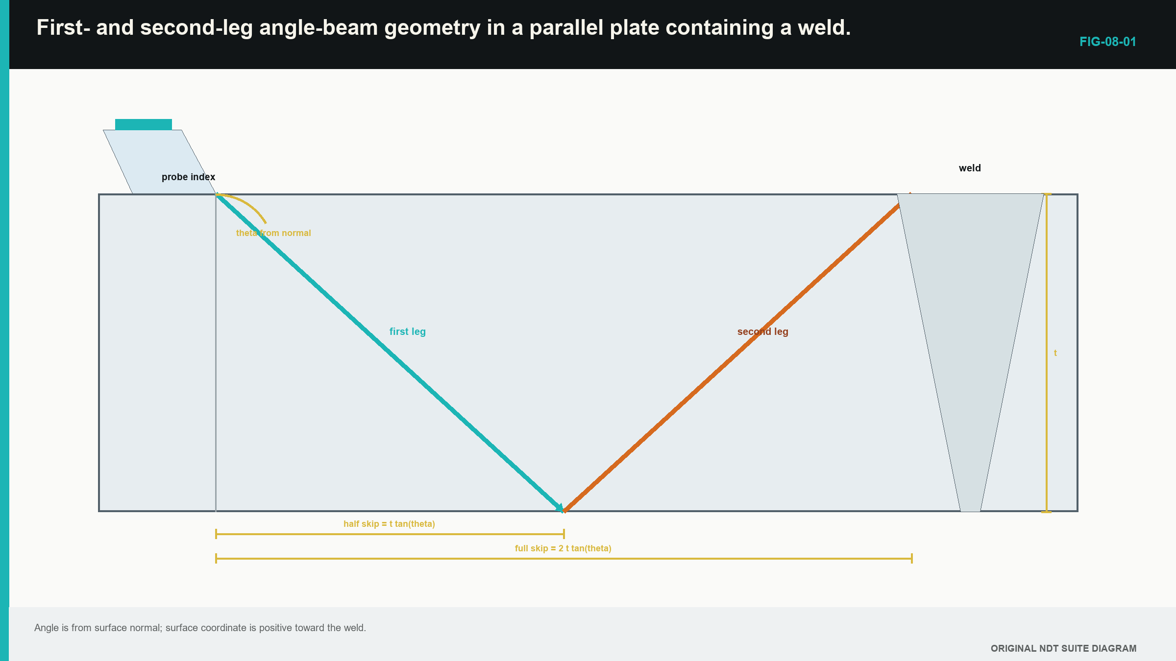
The first leg runs from the probe index to the first back-wall reflection. The second leg runs upward after that reflection. A third leg runs downward again after reflection from the scanning surface.
For plate thickness T, the sideways distance to the first back-wall reflection is commonly called the half-skip distance. The distance to return to the scanning surface after two legs is the full-skip distance.
Tangent connects sideways and downward parts of the right triangle. In words:
half skip = thickness × tangent of the angle
full skip = twice the half skip
| (8.2) Skip distances · EQ-08-02 Where: H = half-skip surface distance (m); F = full-skip distance (m); T = plate thickness (m); theta = refracted angle from surface normal Model limits: parallel planar surfaces and specular reflection |
|---|
The sound path to the first back wall is the thickness divided by the cosine of the angle. In words:
first-leg path to back wall = plate thickness ÷ cosine of angle
| (8.3) First-leg path to back wall · EQ-08-04 Where: S_backwall = one-way sound path to back wall (m); T = thickness (m); theta = refracted angle from normal Model limits: parallel surfaces and a straight central-ray model |
|---|
This value is a fast leg check. If a response sound path is longer than the first-leg back-wall path, the ray has already reflected in the simple model.
Before using any coordinate equation, compare the displayed sound path with the path to the first back wall. A smaller value can fit the first leg. A larger value cannot. This order catches an impossible depth before several neat calculator steps make it look respectable.
| Worked example · Selecting the correct path leg WE-08-02 Given: Plate thickness is 25.0 mm. Refracted angle is 60.0 degrees. A response occurs at 60.0 mm sound path. Find: Whether the central-ray path reflected from the back wall before reaching the response. Steps: Find the first-leg path to the back wall. S_backwall = 25/cos(60 degrees) = 25/0.5 = 50.0 mm The response path is 10.0 mm longer than the back-wall path, so it lies on the second leg. Over that extra path, upward vertical travel is: 10.0 cos(60 degrees) = 5.0 mm Depth from scanning surface is 25.0 - 5.0 = 20.0 mm. Answer: The model places the response on the second leg at 20.0 mm depth. What this tells you: Treating the full 60.0 mm as first leg would give 30.0 mm depth in a 25.0 mm plate. The leg check catches that impossible answer. Common mistake: Using the first-leg depth formula without comparing sound path with the back-wall path. |
|---|
The next figure shows first and second legs beside a weld. Notice that surface distance continues to increase after reflection.
8.3 The probe label is a starting point
A probe marked 60 degrees is designed to produce about that refracted angle under stated conditions. Wear, wedge temperature, material velocity and construction tolerance can change the actual result.
The probe index can be established using a known radius or other suitable reference target. The point of maximum response is related to the exit location. Refracted angle can be estimated from the known reflector position and measured probe position.
These measurements have finite width because the beam and reflector are not infinitely thin. Repeating the check helps show placement variation. Checking from more than one direction can reveal wedge asymmetry or a reading bias.
Wedge wear moves the index and can change the physical incident angle. Wedge speed changes with temperature, which changes refraction. A long sound path turns a small angle error into a larger coordinate error. An index error adds directly to surface position.
Verification compares the complete system with known geometry. It can establish usable time base, index, angle and response. It does not prove that every natural discontinuity orientation will be detected.
For a beginner, the check can be recorded as a short chain. Mark the index on the wedge. Place that mark against the reference scale. Move the probe to the maximum response from the known target. Record the probe position and the displayed path. Repeat the placement before changing any setting. The spread between placements shows how consistently the point can be found.
If the response is broad, do not choose one edge simply because it gives the preferred angle. Use the stated reference method, find the same response feature each time and record the usable result. If the check cannot be repeated, the later weld coordinate cannot be more reliable than the check that created it.
If an end check changes, the affected claim depends on the change. A timing change affects location. An amplitude change affects sensitivity comparison. An angle or index change affects location and coverage. The record must identify which data interval could be affected.
8.4 Start weld interpretation with geometry
Before naming a weld response, build a simple geometry picture. Record wall thickness, bevel shape, root position, cap, backing, counterbores and the scanning surface. Establish the probe index direction and component coordinate.
Known weld geometry can give strong echoes. A root corner can return sound. A cap edge can create a path. Backing or a counterbore can produce a repeatable signal. These are not flaws, though relevant discontinuities can exist beside them.
A planar lack-of-fusion condition is directional. Its face may return strongly only when a beam meets it at a favourable angle. Rounded porosity can scatter over a wider direction range, though real morphology varies.
Probe movement supplies evidence. Moving toward and away from the weld changes the modelled intersection. Small sideways or orbital movements change direction on the reflector. Scanning from another side or with another angle can test a second path.
A simple weld sketch should travel with the A-scan. Draw the scanning surface, near and far weld toes, root, cap and any backing. Add the probe index and beam direction. Then place the calculated response on that picture. The sketch does not prove its cause, but it makes a geometric explanation testable.
For example, a response may appear at the calculated root position. Move the probe a little toward the weld. A genuine path-related response should change in a way that fits the new intersection. A coupling disturbance may change without a sensible geometric pattern. A cap echo may follow the cap edge. Recording that movement is more useful than saving only the highest peak.
The words used at this stage should match the evidence. “Repeatable response at the modelled root region” is a careful observation. “Root crack” is a classification that needs more evidence and authority. Learning to keep those two statements separate is part of ultrasonic skill, not timid report writing.
The Level 1 task is not independent flaw classification. It is to state that a response is valid, locate it under a declared model, compare it with known geometry and describe how it changes with movement.
8.5 Step up preview - paths beyond the second leg
Longer sound paths can reflect again from the scanning surface and enter a third leg. Later levels use a mirrored-plate drawing to fold these paths back into the real plate while keeping the total surface distance and leg number. The physical history still matters because every reflection can change the response.
Level 1 calculations stop at the first and second legs. The later-leg folding examples move to Level 2, where the method is taught and assessed. A Level 1 learner only needs to recognise that a path beyond two legs needs a later-leg method rather than forcing it into a first-leg triangle.
8.6 Step up preview - skew and a third coordinate
A weld cross-section shows surface distance and depth. A real beam may also point along the weld rather than directly across it. That sideways rotation is called skew, and it needs a second surface coordinate before a three-dimensional location can be claimed.
Level 2 develops the coordinate convention and practical skew plotting. Level 3 develops curved-component datums and uncertainty. The three-coordinate equation moves with that material. No three-coordinate calculation is assessed in Level 1.
8.7 Step up preview - a real beam has width
The central ray is a useful direction line, but the probe sends and receives over a region around it. A small reflector can therefore respond without sitting exactly on that line. Probe movement helps show the useful response region, so a calculated central-ray point should not be reported as the exact reflector centre.
Level 2 develops beam profiles, amplitude-drop contours and reference-target comparisons. Those contours are not universal detection boundaries because target shape and direction matter. Level 1 keeps the simple limitation: calculated coordinates are modelled locations, not microscopic photographs of the reflector.
8.8 Building a careful first weld case
Consider a repeatable response near the predicted weld root. A structured Level 1 explanation proceeds in layers:
- Confirm that coupling, time base and response are stable and unsaturated.
- Establish probe index, refracted angle and sound path.
- Select the correct leg using plate thickness.
- Calculate a plausible coordinate.
- Compare that position with root, fusion face, cap, backing and other geometry.
- Observe response movement and, where available, use another direction.
- State which causes are consistent and which evidence would separate them.
This order is intentionally slow. It prevents a strong peak from becoming a flaw name before the path has even been checked. On an instrument, first freeze or save the relevant A-scan. Record the probe position without moving it. Then complete the geometry sketch. If the result is impossible, return to the time base, index, angle and leg choice rather than adjusting the drawing until the answer fits.
A response that follows root geometry from symmetric scans can support a geometric explanation. A strongly directional response that lies on a fusion face can support a planar-reflector hypothesis. Neither pattern alone supplies acceptance or a reliable height.
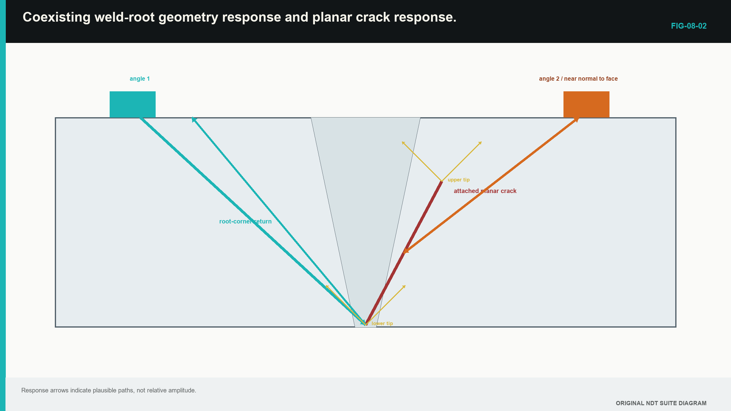
Geometry and a relevant discontinuity can coexist. A crack can begin at a root that already gives a normal corner response. One part of the signal may follow root geometry while another extends away or behaves differently with angle. Automatically deleting everything inside a “root zone” can hide relevant evidence.
The figure shows a root corner and an attached planar crack as two possible response mechanisms. Notice that the arrows describe plausible paths, not guaranteed amplitudes.
Surface curvature, thickness change, anisotropy and temperature can make a flat constant-speed model inaccurate. Beam width limits location. Confidence in the final coordinate cannot exceed confidence in angle, index, leg and echo identity.
The same reasoning carries into PAUT. A sector scan shows many angle laws together, but every response still depends on time, path, field and reflector interaction. Colour and automatic plotting speed up the geometry. They do not remove the assumptions.
A useful beginner record contains the plate thickness, probe identity, marked index, established angle, beam direction, sound path, chosen leg and calculated coordinate. It also retains the A-scan and probe position. Another person can then rebuild the same simple model and see where observation ended and interpretation began.
The angle-beam geometry and verification foundation in this chapter follows the cited international training source. [R001]
In plain words
- Probe index is the surface starting point for the modelled central ray.
- Sound path splits into depth and surface distance by simple trigonometry.
- A path longer than the first back-wall path has entered a later leg.
- Half skip reaches the back wall; full skip returns to the scanning surface in the simple plate model.
- Probe angle and index must be established rather than trusted only from the label.
- Later-leg paths need a separate folding method taught in Level 2.
- A real beam occupies a region around the central ray, so a coordinate is not an exact point photograph.
- Weld geometry, movement and alternative directions are needed before naming a response.
Key terms
- Probe index: declared surface entry reference for the central ray.
- Sound path: length travelled along the beam model.
- Leg: section of path between surface reflections.
- Skip: surface distance associated with angled path legs.
- Central ray: convenient line used to represent the middle of a finite field.
Key relationships
- z = S cos(theta) and x = S sin(theta): first-leg depth and surface distance.
- H = T tan(theta) and F = 2T tan(theta): half- and full-skip distances.
- S_backwall = T/cos(theta): sound path to the first back-wall reflection.
Common mix-ups
- Angle from the normal is not angle from the surface.
- Sound path is not the same as depth.
- A second-leg response cannot be located with an unchanged first-leg depth formula.
- Nominal probe angle is not automatically the actual angle in the component.
- A central-ray coordinate is not the complete beam region.
Bridge to Part II
Part I has built the physical and practical foundation: materials, waves, interfaces, probes, A-scans, thickness and one angle-beam path. Part II turns those individual ideas into technique. It develops beam fields, calibration, reference sensitivity, product and weld geometry, coverage, interpretation and sizing without assuming that the learner arrived wearing an engineering degree.
Sources and further study
- [R001]
CLASSROOM LAB · INTERACTIVE
Try the beam and A-scan
Connect probe position, beam path and displayed response. This is a simplified teaching model, not a calibration or inspection calculation.
Open the full classroom lab ↗Study and revision only. This is not an approved inspection procedure, acceptance criterion or qualification.