From a Valid PAUT Response to a Restrained Result

Why this matters

The most dangerous PAUT mistake is not missing a colour. It is giving a convincing colour the wrong physical story. Interpretation compares competing explanations using valid data, raw A-scans, geometry, law dependence and probe movement. Sizing comes later and only through a supported method. Evaluation comes later again, using the supplied acceptance source. This chapter starts with three common cases so the analysis sequence stays connected to real evidence rather than becoming a list of document-control terms.

What you already need

• Common PAUT views can be traced to A-scans, laws and encoded positions.
• Corrected locations depend on wedge, material and component models.
• Coverage and data quality must be established before interpretation.
• Beam width, side responses and reflector orientation affect screen appearance.
• Calibration and performance checks protect different parts of the evidence.

What you will learn

• Apply a data-validity gate before interpreting a response.
• Compare geometric, coupling, system and material explanations.
• Corroborate a response across A-scans, laws, views and probe movement.
• Separate characterisation from sizing and evaluation.
• Compare supported measurements with a supplied controlled criterion.
• Record evidence, limitations and conclusion without claiming more than the data show.

Words you will meet

• Indication: observable examination evidence that may need interpretation.
• Non-relevant indication: a real response source outside the discontinuity class being evaluated.
• Relevant indication: a response associated with a condition requiring evaluation under the governing rules.
• Characterisation: assessment of likely physical type, orientation or relationship.
• Sizing: estimation of one or more dimensions using a stated method.
• Evaluation: comparison of established information with applicable criteria.
• Disposition: authorised status or action assigned after evaluation.

36.1 Case 1: a continuous response near the weld root

An encoded weld scan shows a response that follows the root line over much of the pass. It appears over neighbouring apertures and changes position in a way that broadly matches probe movement. A drawing shows possible internal mismatch. One local segment, however, extends away from the predicted geometric line and responds differently from a second direction.

The whole feature should not be labelled either “root geometry” or “lack of penetration” from position alone. The continuous part is consistent with a geometric source, but the local extension needs separate analysis. Inspect the contributing A-scans, compare sound path with actual root geometry, observe angular behaviour and retain the second-direction evidence.

The restrained result can contain two parts. One region may be recorded as a likely geometric response with its basis stated. The local extension can remain relevant for supported characterisation, sizing and evaluation. If the as-built geometry is unavailable, uncertainty in the explanation remains visible rather than being removed by confident wording.

This case teaches the first rule: expected location is supporting evidence, not proof of source.

36.2 Case 2: a dark patch in a C-scan

A C-scan contains a low-amplitude patch beside a bright edge. The patch could be interpreted as a low-reflecting material region. The linked A-scans show a different pattern: the back-wall response falls at the same positions, interface noise rises and some traces contain intermittent drop-out. The patch follows a rough surface band.

This is evidence of degraded or invalid coupling, not evidence that the material is free of discontinuities. It is also not automatically a “false flaw.” The map has truthfully displayed the selected gated value; the false step would be treating that value as a component condition without checking how it was produced.

Bound the affected coordinates, restore the controlled surface or coupling condition, confirm the required checks and reacquire with overlap when permitted. Preserve both datasets. The replacement file does not erase the original acquisition problem.

This case teaches the second rule: absence of a valid ultrasonic response is not proof of clear material.

36.3 Case 3: a repeatable off-axis response

A bright response appears over several laws at a location not supported by the main-beam geometry. It repeats as the probe moves, which initially makes it look like a stable discontinuity. The response also appears at a similar offset from a known geometric reflector and changes strongly when the aperture or steering range changes.

Possible explanations include a side or grating response, a mode-converted path, an internal wedge echo or an incorrect geometry model. Repeatability proves that the mechanism is stable; it does not prove that the main-lobe centreline located it correctly.

Compare raw timing, law dependence, probe movement and predicted alternative paths. Change one approved analysis or rescan variable at a time and preserve the original data. A response that moves according to an alternative path model can support that explanation. Visual resemblance to an artefact atlas is weaker than a controlled change that predicts the observed movement.

This case teaches the third rule: repeatability strengthens an observation but does not select its physical explanation.

36.4 First gate: confirm that the data are valid

Before interpreting any response, confirm the relationship among file, component, scan and setup. Check that calibration and performance evidence covers the acquisition interval. Confirm required scan extent, encoded continuity, material and wedge inputs, law identity and known field limitations.

Inspect the data state. Establish whether waveforms are RF or rectified, whether amplitudes are clipped, which filters or smoothing are active and whether the current view contains interpolation or correction. Confirm that the relevant gate includes the response.

Check coupling and background behaviour over the feature. Compare start and end coordinates with the scan plan. Note excluded areas, interruptions and any failed checks. If the required volume was not scanned or the data are invalid, report the affected evidence boundary before attempting to classify the component.

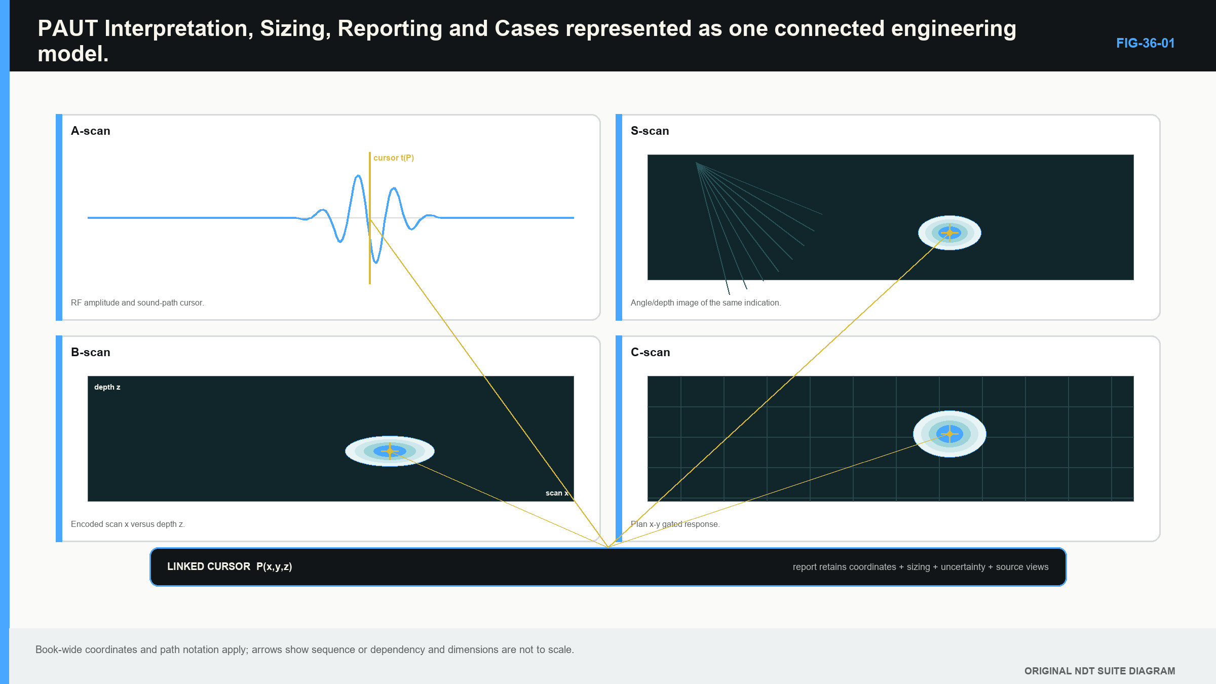
The following figure places the validity gate before every later decision. The arrows return from each spatial view to the contributing A-scan and law. [R018] [R019]

36.5 Use decision labels carefully

An indication is observed examination evidence. It can come from a material condition, normal geometry, coupling, electronics or processing. A discontinuity is a physical interruption or variation in material continuity or configuration. The word defect is often reserved for a condition that fails applicable criteria, although the controlled document's definition governs.

Keep the work stages separate:

1. Detection: observe a response.
2. Localisation: establish its coordinates and sound-path relationship.
3. Interpretation: compare physical explanations for its source.
4. Characterisation: describe likely orientation, form and component relationship.
5. Sizing: estimate a required dimension through a supported method.
6. Evaluation: compare the established information with the supplied criteria.
7. Disposition: assign an authorised status or action.

A strong detection can be poorly located. A well-located response can remain ambiguous. A likely planar condition can be detected without its height being measurable. A measured value does not decide acceptance until the applicable criterion is used.

The labels false, non-relevant and relevant depend on the controlling terminology. A false indication can be an apparent component feature produced by electronics, processing, coupling or a misleading acoustic path. A non-relevant indication can arise from real intended geometry. A relevant indication requires evaluation; it is not automatically rejectable.

36.6 Build competing explanations

Start with the response facts: component coordinate, sound path or time, law range, amplitude behaviour, extent along scan and index, and relation to known surfaces. Then list plausible explanation families.

Geometry explanations include cap, root, counterbore, backing, mismatch, thickness transition, curved surfaces and attachments. Acoustic-path explanations include reflection, skip, mode conversion, side or grating response and wedge echoes. Acquisition explanations include coupling loss, saturation, gate selection, encoder misregistration and channel faults. Material explanations include intended interfaces, coarse structure and credible discontinuities.

Use process knowledge to rank rather than declare. A response on a fusion face can be consistent with lack of fusion, but bevel geometry can also occupy that location. A cluster in cast material can be consistent with porosity or shrinkage, while coarse structure can create distributed noise. A service crack can be rough, branched and orientation-sensitive.

For each leading explanation, identify an expected observation. Geometry should follow a predictable coordinate or path as the probe moves. Coupling loss often affects back-wall or interface behaviour. A specular plane may peak over a narrow angular band. An off-axis response can maintain a characteristic offset from a strong reflector.

The explanation that best accounts for several independent observations is stronger than one based on colour and location alone.

36.7 Corroborate across waveform, law, view and movement

Return to the underlying A-scan. Check echo shape, time, clipping, noise and gate interaction. Follow the same cursor into the sector and encoded views. Verify that the feature is not created by interpolation, smoothing or a wrong corrected geometry.

Observe how the response rises, peaks and falls as the aperture or probe passes. Compare neighbouring laws and note the rational angular band over which it appears. A response on one isolated law can be real, but it needs careful checking. A response over many laws can reflect a broad beam or rough target rather than a large object.

Compare forward and reverse travel where equivalent acquisition is supported. Use an opposite direction or complementary skew when the technique includes it. Agreement among different physical sensitivities can strengthen the case; repeated views derived from the same A-scans are not independent confirmation.

Multi-view research shows that direct, reflected and mode-converted paths can respond differently to target orientation and structural noise. It also shows that combining views can introduce artefacts. Use view diversity as bounded evidence, not a vote in which the brightest images win. [R018] [R019]

When a controlled rescan is used, state the hypothesis and the changed variable. Preserve the original production data. A rescan with different angle, position or skew is useful when its predicted outcome can separate explanations.

36.8 Characterise only as far as the evidence supports

Characterisation describes the most defensible physical understanding. It can address planar or volumetric behaviour, likely orientation, surface connection, position in the weld, continuity and grouping.

Use language matched to evidence. “Response consistent with a fusion-face planar condition” states both observation and interpretation. “Crack” claims a specific physical mechanism and needs correspondingly stronger support. “Unknown relevant response” is appropriate when the data support evaluation but not a reliable type.

Keep coordinate meanings explicit. Distinguish scan-axis length from beam-spread length, through-wall height from sound-path extent, depth below the surface from distance along the beam, and one connected response from separate responses that may interact under the criteria.

Confidence is not a decorative word. State why the interpretation is strong or limited. Agreement with verified geometry, complementary direction and stable raw timing can increase confidence. Missing as-built dimensions, poor signal-to-noise ratio or dependence on one processed view reduce it.

36.9 Size with a stated supported method

Sizing methods answer different dimension questions and carry different assumptions. An amplitude-drop method finds positions where response crosses a stated level relative to a peak. It depends on beam shape, target orientation, noise, saturation and the selected drop rule.

A beam-boundary method relates response endpoints to a characterised field boundary. It does not trace the physical discontinuity edge directly. Tip-diffraction or time-of-arrival methods require identifiable and correctly paired tip signals with enough resolution. Encoded length sizing depends on scan increment, beam footprint, encoder performance and endpoint rules.

Never size from a clipped signal. If an approved analysis method permits gain change, preserve the original acquisition and record the analysis setting. DAC or TCG provides an amplitude reference through path; it does not turn response height into real flaw dimensions.

If the technique is supported for detection but not the required sizing task, report the supported observation and use the controlled escalation route. A decimal result is not made defensible by adding another decimal place.

The original chapter's formal combined-uncertainty equation and tip-to-tip uncertainty example have been moved to the Level 3 metrology treatment. Level 2 still records method resolution, repeatability and important location limitations, but it does not depend on covariance-free uncertainty mathematics.

36.10 Compare with the supplied acceptance source

Evaluation begins only after the relevant information has been established. Identify the controlled acceptance source and its applicable component, material, joint, service and examination conditions. The PAUT method document and the product acceptance source may be different documents.

Extract the variables the criterion actually uses. They may include amplitude class, length, height, position, surface connection, separation, interaction, thickness or characterised type. Apply the stated units, rounding and grouping rules. This study chapter supplies no universal threshold.

Record the measured or characterised inputs used in the comparison, the exact source and revision, the applied rule, important limitations and the outcome. A relevant indication can be acceptable or unacceptable depending on that controlled comparison.

A Level 2 examiner works within assigned scope. Changing acceptance criteria, waiving missing coverage or granting an engineering concession is a different authority. The technical report should not blur observation, evaluation and authorised disposition.

36.11 Build a traceable result

A competent reviewer should be able to connect the result back to the component, configuration and raw evidence. Record the component and examination area, data file and setup identity, law group, coordinate convention, linked A-scans and views, calibration and check status, relevant processing, response measurements, interpretation basis, sizing method, acceptance source and limitations.

For every reportable response, state units and coordinate meaning. “35 mm” may mean depth, sound path, scan position or length. A screenshot should retain axes, cursor values, file identity and processing state. It should link to the original data rather than becoming an orphaned picture.

Use factual scope language. “No reportable indications observed in the successfully examined volume” states an evidence-limited result. “Component free of defects” claims knowledge beyond what one examination can support.

When data are reacquired, preserve the relationship between original and replacement files. When a released coordinate is corrected, retain revision history and explain what changed. Traceability protects the technical reasoning, not only the paperwork.

Example of a restrained indication entry

An analysis entry can be written in the same order as the evidence:

A repeatable response was observed from scan position 124.0 mm to 141.5 mm in the stated component coordinate system. It is present over laws 48-56 and is strongest on the linked 52-degree A-scan. Corrected depth varies from 18.2 mm to 20.0 mm under setup PA2-WELD-A. Calibration and end checks covered the acquisition interval.

The response lies adjacent to the near-side fusion face and is consistent with a planar fusion-face condition. The stated 17.5 mm scan-axis length was obtained using the approved endpoint rule; through-wall height was not established. The indication was compared with the identified acceptance source using the recorded length and characterisation. The result and any disposition authority are recorded separately.

This wording does several useful things. It begins with observable position and law evidence. It identifies the setup and valid-data basis. It uses “consistent with” for the interpretation. It states the sizing method's dimension and admits the dimension not established. It separates comparison with criteria from the authority that assigns final status.

A weaker entry would say only “17.5 mm lack of fusion, reject.” That sentence hides coordinate convention, raw response, setup, sizing basis, acceptance source and authority. Its confidence comes from compression rather than evidence.

The exact report fields follow the controlled system. The study habit is universal: make every technical noun traceable to an observation, method or source, and make every limit visible.

When evidence is mixed, the entry can remain open rather than forcing an early flaw name. Record the observed response and the competing explanations, then state which additional view, geometry measurement or controlled rescan could separate them. An unresolved result with a clear evidence need is more useful than a confident label that another reviewer cannot reproduce.

The conclusion should be as short as the evidence permits, not as short as the reporting form encourages. Compression belongs after traceability has been preserved.

Keep the original observation available beside any shortened report wording. A reviewer should be able to expand the summary back into the law, waveform, coordinate and criterion chain without guessing.

Step up: governance, uncertainty and release

Formal quality assurance, document hierarchy, validation records, uncertainty budgets, approval roles and change governance move to Chapters 42, 45 and the engineering part. The Level 2 sequence remains practical: valid data, restrained interpretation, supported sizing, comparison with supplied criteria and a traceable record. None of the moved topics is an assessment prerequisite here.

In plain words

• Interpretation begins only after data validity and coverage are checked.
• Position and repeatability support an explanation but do not prove it.
• Raw A-scans, law behaviour, probe movement and geometry should be compared together.
• False, non-relevant and relevant are different decision labels.
• Characterisation states the most defensible physical explanation and its limits.
• Sizing needs a method supported for the required dimension and conditions.
• Evaluation compares established information with a supplied controlled criterion.
• A report must preserve the path from raw evidence to restrained conclusion.

Key terms

Indication; discontinuity; false indication; non-relevant indication; relevant indication; interpretation; characterisation; sizing; evaluation; disposition; traceability.

Key relationships

• valid file + valid calibration + complete coverage -> evidence suitable for analysis;
• location + waveform + law dependence + movement + geometry -> interpretation support;
• characterised response + qualified method -> supported size estimate;
• supported information + applicable acceptance rule -> evaluation;
• evidence, assumptions, limitations and source -> traceable result.

Common mix-ups

• Repeatable does not automatically mean correctly located by the main beam.
• Missing signal is not evidence of clear material when coupling is invalid.
• Relevant does not mean rejectable.
• TCG-corrected amplitude is not physical flaw size.
• A report image is not a substitute for the original data and setup identity.

Bridge to Part V

Part IV has completed the Level 2 crossover from one conventional A-scan to array elements, focal laws, groups, displays, encoded position, calibration, coverage and interpretation. Part V revisits the same chain at Level 3 depth. It adds field theory, detailed timing, performance design, validation and technical responsibility without changing the pulse-echo foundation.

Sources and further study

• [R018]
• [R019]