
CHAPTER 3 · FMC / TFM / PCI Level 2
PAUT Foundations Reframed
In this chapter · 14 sections
Learning outcomes
After completing this chapter, the learner should be able to:
explain how element pitch, aperture, delay laws, steering and focusing form a PAUT beam;
distinguish beamforming during PAUT acquisition from pairwise FMC acquisition;
compare a PAUT focal law with pixel-specific TFM reconstruction delays;
predict how aperture, element directivity and steering limits affect both methods;
identify calibration and verification controls that transfer from PAUT;
identify amplitude controls that transfer only to qualified amplitude reconstructions;
compare the data retained by conventional PAUT and FMC; and
select evidence needed before replacing or supplementing an approved PAUT technique.
Crossover map
| PAUT foundation | FMC/TFM connection | Transfer condition |
|---|---|---|
| Element pitch and array layout | Define pair positions and spatial sampling | Actual element coordinates and probe identity must be correct |
| Active aperture | Defines available transmit-receive geometry | Pair selection and sparse acquisition must be documented |
| Delay law | Provides the intuition for time alignment | TFM applies pair delays during reconstruction rather than one focal law at acquisition |
| Steering and focusing | Explain aperture and orientation sensitivity | TFM performance still varies across the ROI and path |
| Grating/side lobes | Remain possible image artefact sources | Must be assessed for the actual array, frequency, aperture and view |
| Wedge and index calibration | Feed the travel-time and coordinate model | All geometry and velocity inputs must match the reconstruction |
| Encoded scan | Connects data to physical position | FMC adds much larger per-position data and integrity demands |
| Reference sensitivity and TCG | May support amplitude-TFM where qualified | Do not transfer to amplitude-free PCI |
The array has not changed its physics
A phased-array probe contains multiple individually connected elements. Element geometry, centre frequency, bandwidth, pitch and aperture determine what wavefields can be produced and received. The same physical array can support conventional PAUT laws, FMC or other acquisition strategies if the instrument, probe wiring and procedure allow them. The array does not become a different transducer merely because the processing method changes.
Pitch is the centre-to-centre spacing between adjacent elements. Element width is the active dimension of one element in the steering plane. Kerf is the separation between active elements. Aperture is the active collection of elements used for a transmit or receive event. A larger usable aperture can improve lateral resolution at appropriate depths but can also increase sensitivity to geometry, directivity and coupling variation.
Each element has finite directivity. It does not transmit or receive equally in every direction. At large steering angles, outer elements or widely separated pairs may contribute little useful energy to a target. A processor can include a pair mathematically even when the acoustic path lies outside effective element directivity. Technique development must therefore consider usable aperture, not only the number of available channels.
How a PAUT focal law works
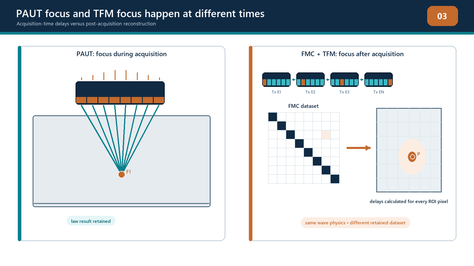
In a conventional PAUT focal law, a group of elements transmits with controlled time delays. Their individual wavelets interfere to form a steered or focused wavefield. Reception may apply a corresponding set of delays before the signals are combined. A sectorial scan repeats this process with different angle laws. A linear scan moves an active aperture electronically along the array. Other law sequences combine steering, focus and aperture movement.
The law is applied during acquisition. The stored beam data have already been combined according to that law unless the instrument separately retains elementary channel information. Changing the focus or angle later may require reacquisition because the original pairwise data were not stored.
PAUT terminology remains useful because TFM also relies on timed alignment across an aperture. The important difference is where the alignment occurs and what information remains available.
How FMC changes the acquisition
In a conventional FMC cycle, one selected element transmits while the selected receive elements record separate A-scans. The next transmitter fires and the receive process repeats until the acquisition matrix is populated. No single PAUT focal law is needed to steer a multi-element transmit beam in the basic sequence. The retained elementary traces can later support multiple reconstructions, subject to the data, model and instrument limits.
This flexibility has costs:
many more A-scans are recorded at every encoded position;
acquisition and processing time can increase;
storage and transfer requirements increase;
channel timing and geometry errors can affect many reconstructed pixels;
raw data and metadata need stronger configuration control; and
the availability of multiple views can create more artefact paths and interpretation burden.
FMC is therefore not automatically better than PAUT for every task. Conventional PAUT can be efficient, well qualified and entirely adequate. FMC/TFM can add value when post-acquisition focusing, multi-path reconstruction, improved region coverage or complementary evidence is needed and demonstrated.
From a focal point to a reconstruction region
A PAUT law usually targets a declared angle, focus or aperture behaviour. The beam still has finite width and a depth-dependent response. TFM defines a region of interest and calculates delays for every candidate pixel using each usable transmit-receive pair. This is sometimes described as focusing everywhere, but three limitations must be retained:
focusing is calculated only inside the selected region;
it is calculated only for the chosen path and velocity model; and
resolution and sensitivity still vary with wavelength, aperture, element directivity, depth and reflector orientation.
If a target is beyond the effective aperture or outside a mode's acoustic coverage, a small pixel grid cannot make it visible. If the model uses the wrong surface or velocity, the delays can align the wrong samples. If the selected path is physically implausible, a bright pixel can still be an artefact of another wave path.
The crossover technician should replace the question Where is the focal depth? with four questions:
What region is being reconstructed?
Which pairs contribute meaningfully at this pixel?
Which propagation path is assumed?
What demonstrated point-spread and sensitivity behaviour exists at this location?
Steering, lobes and spatial sampling
Grating lobes are additional beam directions caused by periodic element spacing and phase relationships. Side lobes are lower-amplitude off-axis responses associated with a finite aperture and weighting. Both can generate responses that reconstruct away from the true reflector location. Their behaviour depends on pitch-to-wavelength ratio, steering, frequency content, aperture, element directivity and weighting.
Do not rely on one universal steering-limit formula without defining its conventions and assumptions. Use a validated array model and representative targets for the selected probe, wedge, material and mode. In TFM, assess the transmit and receive geometry across the full region rather than checking only one conventional central beam.
Apodisation or pair weighting can reduce some lobe contributions at the cost of sensitivity or resolution. Excluding weak or geometrically poor pairs can improve an image, but the change becomes part of the technique. A visually cleaner result is not enough; the qualified performance and retained settings must support the choice.
Receive focusing and dynamic behaviour
Some PAUT systems apply dynamic receive focusing or other post-processing to beamformed data. This can improve focus over depth but does not make the acquisition equivalent to a complete FMC dataset. The system may still have combined channel information according to selected laws.
Likewise, some advanced instruments use plane-wave, sparse or compressed acquisitions to improve speed. They can produce TFM-like or coherence images, but their data structure and performance differ from full pulse-echo FMC. The manual and report should identify the actual acquisition rather than assigning the broadest available label.
Calibration: what transfers and what does not
Several PAUT controls remain essential:
probe and wedge identification;
element-position and orientation accuracy;
wedge delay or complete wedge-path calibration;
material velocity for each selected mode;
time-base and coordinate registration;
encoder distance and direction;
element/channel activity;
amplitude linearity and saturation control where amplitude data are used;
reference-target traceability; and
pre-use and post-use checks.
However, a successful PAUT wedge-delay and sensitivity calibration does not prove TFM coverage or PCI capability. The advanced technique must also demonstrate the reconstruction geometry, selected paths, region limits, grid, pair aperture and processing. Reference targets should challenge the intended depth range and relevant reflector behaviour, not merely produce one attractive response at the centre of the image.
TCG can compensate a qualified amplitude response for path-dependent loss. It cannot be copied into amplitude-free PCI as an equivalent coherence correction. A technique using both amplitude TFM and PCI should maintain separate verification logic for the two output domains while ensuring they refer to the same geometry and data where intended.
Data retained and decisions postponed
PAUT often makes more decisions before scanning: law angles, focal depths and apertures. FMC postpones some focusing decisions by retaining elementary pair signals. Postponement does not remove responsibility. The acquisition must still cover the required time range, bandwidth, matrix aperture and encoded area. Data omitted during capture cannot be recovered by later reconstruction.
Retaining pairwise data permits a reviewer to:
reconstruct a different justified region or path without reacquiring;
inspect individual traces supporting a response;
compare amplitude and coherence processing; and
test sensitivity to selected reconstruction parameters.
This is valuable only when raw data are retained with complete metadata and protected from uncontrolled alteration. If the instrument stores only derived images, later claims of refocus or independent reconstruction may not be valid.
Field workflow: compare before replacing
When considering FMC/TFM as a supplement or alternative to an existing PAUT technique:
state the inspection limitation or objective that motivates the change;
document the approved PAUT coverage, calibration and evidence baseline;
select an array and acquisition that can support the required TFM paths;
compare effective aperture, orientation coverage, near-surface limits and scan speed;
demonstrate performance on representative targets across the full region;
compare false calls and missed responses, not only best-case images;
control every new essential variable; and
obtain the required technical and document approval before production use.
The goal is not to make TFM look sharper than PAUT on one reflector. The goal is to show that the proposed technique performs the required examination reliably within declared limits.
Practical 3 - Compare PAUT and FMC acquisition
Objective
Demonstrate the difference between a PAUT focal-law record and a pairwise matrix record using the same array and reference targets.
Resources
documented array and wedge;
homogeneous reference block with at least two targets at different positions;
PAUT setup with a justified law set;
FMC or supplied full-matrix dataset; and
worksheet for aperture, data and image comparisons.
Method
Record the probe, wedge, frequency, active elements, velocity and coordinate origin.
Predict which PAUT laws should respond to each target.
Acquire the approved teaching PAUT law set and save its data.
Acquire the FMC sequence over the same physical position and time range.
Compare the number and type of retained traces, acquisition time and file size.
Reconstruct one justified TFM view and compare target positions and point-spread shapes.
Inspect individual matrix traces that contribute to one TFM response.
State which changes can be made after acquisition and which would require reacquisition.
Required evidence
controlled setup summary for both acquisitions;
PAUT law and FMC matrix diagrams;
file-size and acquisition-time comparison;
annotated target images and three contributing pair traces; and
transfer table for calibration and verification controls.
Stop rules
Stop if the array position, wedge model, velocity, time range or target coordinates differ between datasets without being documented. Do not compare image brightness when display domains, gain or normalisation are not equivalent. Stop if either acquisition clips the raw waveform.
Successful completion
The learner explains that PAUT forms selected laws during acquisition while FMC retains elementary pair data for later reconstruction, and does not claim universal superiority for either method.
Common traps
Calling TFM a sharper S-scan. The acquisition, reconstruction and data retained can be fundamentally different.
Assuming every array pair is equally useful. Element directivity, path length, aperture and coupling affect contributions.
Using conventional PAUT calibration as complete TFM validation. The reconstruction region, path and performance also require evidence.
Selecting the maximum available aperture automatically. More pairs can add noise, lobe energy and poorly supported paths.
Treating a sparse acquisition as full FMC. Name the actual matrix and demonstrate its performance.
Comparing colour brightness between PAUT, amplitude TFM and PCI. Confirm units, normalisation and response domain first.
Chapter summary
PAUT and FMC use the same array physics but organise excitation, reception and retained data differently. PAUT focal laws combine delayed element contributions during acquisition. FMC records pairwise signals so selected focusing and path decisions can be applied during reconstruction. TFM flexibility remains bounded by the array, aperture, directivity, waveform quality and acoustic model. PAUT calibration skills transfer, but they must be expanded to verify the matrix, reconstruction region and advanced output. A new image should be adopted because its performance is demonstrated for the examination problem, not because it is visually cleaner.
Study and revision only. This is not an approved inspection procedure, acceptance criterion or qualification.