
CHAPTER 9 · Ultrasonics Level 2
What the Beam Really Covers
In this chapter · 19 sections
Why this matters
A centreline drawn from a probe to a reflector is useful, but it is not the whole beam. On a real plate, the echo can rise or disappear after only a small probe movement. The change may come from beam width, near-field variation, target direction or pulse length. A Level 2 technician needs to connect those effects to practical choices: probe frequency, element size, scan spacing and target depth. This chapter starts with the screen and the component, then adds enough field theory to explain what the technician sees.
What you already need
- A probe sends a pulse and receives returning sound.
- Wavelength is wave speed divided by frequency.
- Gain changes displayed response height but does not change the acoustic beam.
- A centreline ray shows a possible path, not the full sound field.
- Sound path, depth and surface distance are different quantities.
What you will learn
- Explain why echo height can vary inside the near field.
- Compare beam width, divergence and pulse length as separate limits.
- Estimate near-field length and a declared far-field angle.
- Distinguish detectability from axial, lateral and near-surface resolution.
- Use beam evidence to choose scan spacing and check coverage.
- Recognise when a neat ray drawing overstates practical capability.
Words you will meet
- Aperture: the active probe area that sends or receives sound.
- Near field: the region where wave contributions create strong spatial variation.
- Far field: the later region where the main beam spreads more regularly.
- Divergence: the spreading of the beam with distance.
- Resolution: the ability to separate nearby responses.
- Beam map: measured response at known positions through the field.
- Side lobe: a weaker response region away from the main beam.
9.1 Begin with a plate and three equal reflectors
Consider a straight-beam probe on a plate containing three equal small reflectors. They are directly below one another at shallow, middle and deep positions. A centreline drawing passes through all three. The screen, however, may show very different echo heights.
The shallow reflector may lie in a region where parts of the probe face interfere strongly. A movement of one or two millimetres can change its response. The middle reflector may sit near a strong part of the field. The deep reflector may give a wider but weaker response because the beam has spread and the path has added loss.
This behaviour does not mean the reflectors changed size. It means the probe creates a field with width and structure. Every point across the active face sends a small contribution. Those contributions reach a location with different travel times. They can reinforce each other or partly cancel.
The active face is called the aperture. A ray drawn through its centre is a convenient geometry tool. The actual beam occupies a region around that ray.
9.2 Near field in plain language
Close to an unfocused probe, sound from different parts of the aperture has not yet settled into a simple spreading pattern. Some locations receive contributions that add strongly. At other locations, contributions partly cancel. This varying region is the near field.
Near field is not the same as dead zone. Dead zone is the early time or shallow depth hidden by the transmitted pulse, ringing and receiver recovery. Near field is an acoustic field region in which echo response can vary with position.
For an ideal flat circular aperture, the approximate near-field length increases with aperture diameter and decreases with wavelength. In words:
near-field length is approximately aperture diameter squared divided by four wavelengths
| (9.1) Approximate circular-piston near-field length · EQ-09-01 Where: N = approximate near-field length (m); D = active circular element diameter (m); lambda = wavelength in the loaded medium (m) Model limits: flat circular piston, homogeneous isotropic medium, D large relative to lambda, unfocused continuous-wave approximation |
|---|
The equation gives a useful scale. It does not predict every maximum and minimum from a real damped probe. Probe construction, bandwidth, matching layers, load and the reference target all affect the measured response.
| Worked example · Estimate the near-field scale before scanning WE-09-01 Given: A circular probe has an active diameter of 12.7 mm. It operates at 5.00 MHz in steel represented by a longitudinal-wave speed of 5,900 m/s. Find: The centre wavelength and approximate near-field length. Steps: First find wavelength. lambda = c/f = 5,900 m/s / 5.00 x 10^6 Hz = 0.00118 m = 1.18 mm Keep diameter and wavelength in the same unit. N = 12.7^2 / (4 x 1.18) = 34.2 mm Answer: The approximate near-field length is 34 mm. What it means in practice: Equal reflectors inside the first 34 mm may not follow a smooth amplitude trend. Reference responses should be checked at the depths that matter. Common mistake: Treating 34 mm as a sharp boundary where the beam suddenly becomes uniform. |
|---|
9.3 Far-field spreading and beam-width conventions
Beyond the near field, the main beam usually spreads more regularly. This region is commonly called the far field. A larger aperture or a shorter wavelength normally gives a narrower far-field beam. A smaller aperture or longer wavelength normally gives wider spreading.
The phrase “beam edge” needs a rule. Sound does not stop at one line. A beam width might be quoted at a 6 dB drop, at half amplitude, at the first calculated zero, or at another threshold. Two widths can both be correct while describing different contours.
For an ideal uniform circular aperture, the first pressure zero is estimated by the next relationship.
| (9.2) First-zero angle of an ideal circular aperture · EQ-09-02 Where: alpha_zero = half-angle from the axis to the first pressure zero; lambda = wavelength (m); D = active aperture diameter (m) Model limits: uniform circular piston, far field, homogeneous isotropic medium and continuous harmonic component |
|---|
Using the values from the previous example gives sin(alpha_zero) = 1.22(1.18/12.7) = 0.1134. The first-zero half-angle is about 6.5 degrees. That value must not be relabelled as a 6 dB beam edge.
The following figure brings the two regions and several width rules together. Notice that the centreline remains useful, but it does not show the field strength around it.
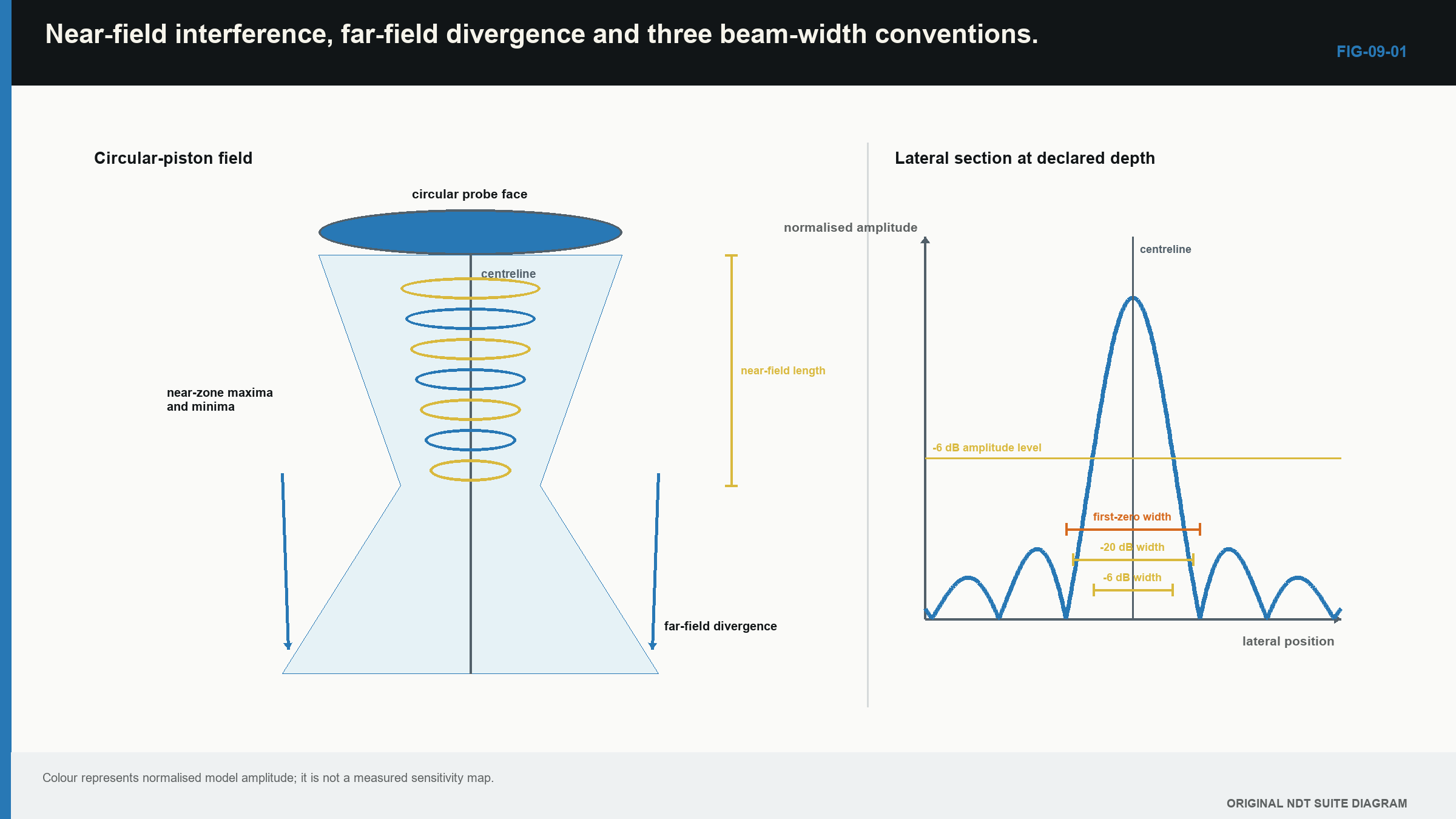
Measured beam maps are normally more useful for a production setup than a single ideal angle. Nominally similar probes can differ through construction, wear and electrical loading. Matching model labels supports identification, but it does not prove identical beam behaviour. [R010]
9.4 Resolution has a direction
Resolution means separating responses that are close together. The word is incomplete unless the direction and depth are stated.
Axial resolution concerns two reflectors placed one behind the other along the beam. It depends strongly on pulse duration. If the first echo is still ringing when the second arrives, the two responses merge.
Lateral resolution concerns two reflectors beside one another across the beam. It depends on beam width at their depth. A narrower field can separate closer side-by-side targets.
Near-surface resolution concerns a reflector close to the entry surface. Initial pulse, interface response, ringing and receiver recovery can hide it.
Detectability is different. A system may show that sound returned from a region without separating two targets in that region. It may also detect a weak diffracted response from a small edge without resolving the edge shape.
The next example connects pulse duration to an axial distance scale.
| Worked example · Relate pulse duration to axial separation WE-09-02 Given: A received pulse envelope lasts about 0.80 microsecond. Use a longitudinal-wave speed of 5,900 m/s. Find: The pulse-echo depth interval represented by that duration. Steps: The time covers outward and return travel, so divide by two. Delta_d = c tau/2 Delta_d = (5,900 m/s)(0.80 x 10^-6 s)/2 = 0.00236 m Answer: The depth interval is about 2.36 mm. What it means in practice: Two equal echoes separated by much less than this are likely to overlap. A weak echo beside a strong one may need even more separation. Common mistake: Calling 2.36 mm the probe’s resolution in every direction and at every depth. |
|---|
9.5 What frequency and aperture change
Frequency affects wavelength. In the same material, higher frequency means shorter wavelength. This can improve separation of small features, but it usually increases loss from absorption and scattering. In coarse material, a lower frequency can give a cleaner usable signal even though its resolution is poorer.
Aperture affects beam shape and probe footprint. A larger unfocused aperture often gives a narrower far-field main beam, greater sensitivity and a longer near field. It can also couple poorly on curvature. A smaller aperture often spreads more widely and fits restricted surfaces better.
These effects interact. The best probe is not simply the highest frequency or largest diameter available. It is the probe that supplies usable signal, resolution and coverage in the target region.
Material loss on the screen combines several effects: beam spread, absorption, scattering, interfaces, coupling and reflector direction. Gain raises received signal and received noise together. It cannot return coherent energy that the material scattered away. Grain scattering becomes important as material structure approaches the wavelength scale. [R009]
9.6 Focus is useful over a region
A focused probe arranges contributions so they reinforce near a chosen depth. The focus is a finite region, not one perfect point. Beam width narrows near the focus and grows away from it.
Focusing can improve local lateral resolution and response. It does not sharpen the whole sound path. Strong focusing can also make the result more sensitive to stand-off, surface shape and velocity error.
For practical selection, compare the focus region with the full target depth range. A narrow focus at the centre of a thick component can leave the near and far parts with weaker coverage. A broader field may be more useful when the target depth is uncertain.
Linear arrays and rectangular probes also behave differently in their two main planes. A long active dimension normally gives a narrower field in that plane. The shorter dimension spreads more widely. One quoted beam width can therefore hide the weaker direction.
9.7 The reference target changes the map
A beam map is not measured without a target. A small sphere, side-drilled hole and flat-bottom hole return sound differently. The recorded width is therefore a complete probe-path-target response.
A side-drilled hole gives a broad useful response across its cylindrical surface. A flat-bottom hole is strongly directional. A small spherical target scatters more broadly. When a map is used for coverage, record the target, scan increment, depth, amplitude rule and normalisation.
Saturation can falsely broaden the peak. Coarse scan steps can miss a narrow lobe. Interpolation can draw a smooth contour between points that were never acquired. Coupling change can imitate field variation.
This does not make beam mapping unhelpful. It makes the conditions part of the result. The international UT foundation used by this book treats beam behaviour, calibration and application as connected controls. [R001]
9.8 From beam width to scan spacing
Scan spacing is a sampling choice. If the declared beam width at target depth is 8 mm and adjacent scan lines are 6 mm apart, the nominal overlap is 2 mm. That is 25% of the stated width.
This overlap is an aid, not a detection guarantee. Sensitivity falls gradually across the field. Target direction can make a reflector quiet even inside the chosen contour. The beam width also changes with depth.
For a simple far-field estimate, beam radius can be projected from a declared half-angle.
| (9.3) Approximate far-field beam radius from an angular convention · EQ-09-03 Where: r = radius from beam axis at axial distance z (m); z = axial distance (m); alpha = declared half-angle using one stated amplitude convention Model limits: straight axis and far-field geometric approximation |
|---|
The important word is declared. A radius calculated to the first zero cannot be compared directly with a measured 6 dB contour.
The following figure separates the three resolution directions. Notice that a short sample pitch does not automatically mean a narrow physical response.
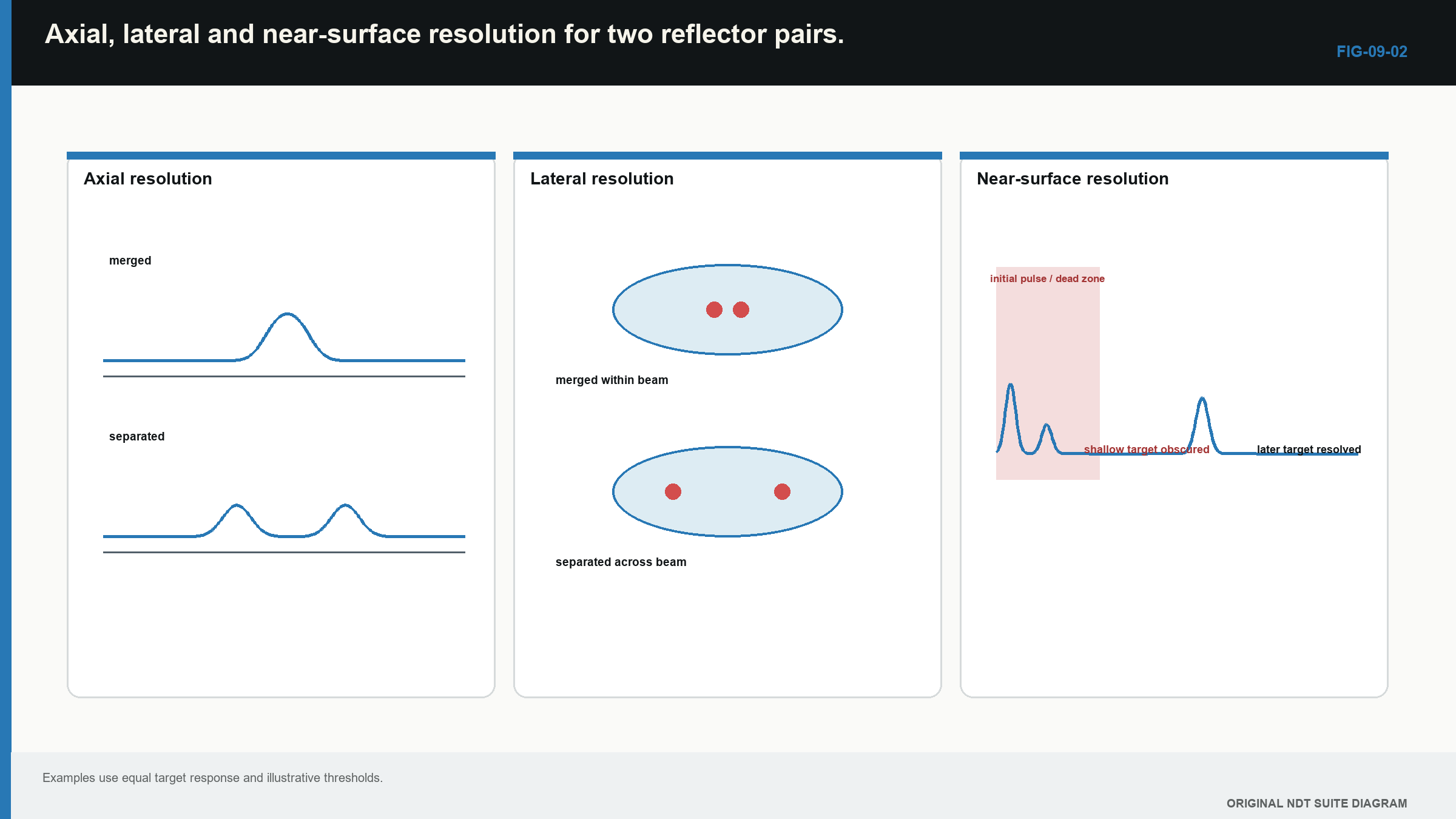
Notice that each resolution direction has a different physical limit; none is proved by small display pixels alone.
| Worked example · Project a declared beam radius and separate it from data spacing WE-09-03 Given: A declared far-field half-angle is 5.0 degrees at an axial distance of 40 mm. Encoded scans are recorded every 0.5 mm, and software displays pixels every 0.1 mm by interpolation. Find: The projected beam radius and the different acquisition and display spacings. Steps: Use the declared angular convention in EQ-09-03. r = 40 mm x tan(5.0 degrees) = 3.50 mm, giving a projected diameter of about 7.0 mm. The acquired scan pitch remains 0.5 mm. The interpolated display pitch remains 0.1 mm. Answer: Projected beam radius is about 3.5 mm, acquired pitch is 0.5 mm and displayed pitch is 0.1 mm. What it means in practice: The radius is an ideal geometric estimate using the stated angle. Smaller pixels make the image smoother but do not narrow the physical beam or prove 0.1 mm resolution. Common mistake: Mixing a first-zero or other model radius with a measured 6 dB width, then reporting display pixel spacing as physical resolution. |
|---|
9.9 Check coverage where it is weakest
One beam width at one depth does not prove complete volume coverage. Near-field variation, focus and far-field spreading change response through the path. A practical check uses reference targets at representative shallow, middle and deep positions.
The weakest region deserves attention. A reflector at the centre of the beam proves little about its edge. A target normal to the beam proves little about an unfavourable orientation. Remounting and coupling variation should also be observed.
The result is a bounded coverage statement. It identifies which region, target type, depth and scan spacing have supporting evidence. A good coverage plan combines geometry, measured field behaviour and a representative response. The tidy ray drawing is still useful; it simply has to bring the rest of the beam with it.
In plain words
- A probe sends sound through a finite area, so the beam has width and structure.
- Echo height can vary in the near field even when reflector size is unchanged.
- A quoted beam edge is meaningful only when its amplitude rule is stated.
- Axial, lateral and near-surface resolution are different capabilities.
- Higher frequency can improve separation but may reduce penetration in difficult material.
- Scan pitch and display pixel size are not the same as physical resolution.
- Beam calculations guide the setup; measured reference evidence checks the real system.
Key terms
- Aperture: the active area that contributes to transmitting or receiving sound.
- Near field: the region of strong spatial response variation near an aperture.
- Far field: the region where the main field spreads more regularly.
- Divergence: increasing beam width with distance.
- Axial resolution: separation along the beam direction.
- Lateral resolution: separation across the beam.
- Beam map: a measured response pattern made with a stated target and scan rule.
Key relationships
- N = D^2/(4 lambda) estimates a circular probe’s near-field scale.
- sin(alpha_zero) = 1.22 lambda/D estimates one specific far-field angle convention.
- r = z tan(alpha) projects a declared beam half-angle over a distance.
Common mix-ups
- Near field is not near-surface dead zone.
- Beam divergence is not the refracted beam angle.
- Display pixel size is not acoustic resolution.
- More gain does not narrow the beam or improve physical resolution.
- A calculated contour is not a guaranteed detection boundary.
Bridge to Chapter 10
Chapter 9 followed sound through space. Chapter 10 follows the returning signal through the instrument. The next step is to see how range, gain, gates, sampling, filters and pulse rate can preserve useful evidence or quietly distort it.
Sources and further study
- [R001]
- [R009]
- [R010]
CLASSROOM LAB · INTERACTIVE
Try the beam-spread lab
Change frequency and crystal diameter to compare two unfocused probes. This is a simplified teaching model, not a calibration or inspection calculation.
Open the full classroom lab ↗Study and revision only. This is not an approved inspection procedure, acceptance criterion or qualification.