
CHAPTER 38 · Phased Array Ultrasonics Level 3
Building and Checking Focal Laws
In this chapter · 25 sections
Why this matters
A law file can report a focus at the correct component coordinate while an independent plot places the energy somewhere else. The disagreement usually begins before the delay table: a different origin, element order, wedge path, velocity, sign convention or interface solution. Focal-law software hides much of that chain because routine production work needs a usable setup, not a page of equations. A PAUT Level 3 must reopen the chain when designing, transferring or approving a technique. This chapter begins with two elements and one focus, then adds wedges, transforms, tolerances, hardware timing and auditable release checks.
What you already need
- The Level 2 meaning of an active aperture, focal law, refracted angle and focus.
- Sound path divided by velocity gives travel time.
- Element number, probe index and component datum are different references.
- Basic trigonometry and three-dimensional component coordinates.
- The array-field and phase-alignment picture from Chapter 37.
What you will learn
- Explain a focal law as a path-time model rather than a stored beam.
- Calculate relative delays for a homogeneous focus and an ideal steering ramp.
- Describe how a wedge/interface solver finds each physical path.
- Apply and independently test probe-to-component coordinate transforms.
- Evaluate sensitivity to geometry, velocity, temperature and delay quantisation.
- Define the checks and records required to release or transfer a law set.
Words you will meet
- Reference time: common arrival time used to convert path times into relative delays.
- Solver: calculation method that finds a path or parameter satisfying declared conditions.
- Path branch: one physically possible solution among several candidate paths.
- Rigid transform: rotation and translation that relate two coordinate frames.
- Tolerance: permitted or expected variation in an input quantity.
- Sensitivity: change in an output caused by a change in an input.
- Delay quantisation: rounding of an ideal delay to hardware timing steps.
- Conditioning: how strongly small input or numerical changes affect a solution.
- Fiducial: independently known point or feature used to test registration.
- Realised law: delays and active channels actually implemented by hardware.
38.1 Begin with two elements and one arrival time
Imagine two elements in one block of steel. The focus is closer to element 2 than element 1, so sound from element 2 would arrive first if both fired together. To make the pulses meet, delay element 2 by the difference between their travel times. Nothing more mysterious is required for the first focal-law idea.
The common arrival time is the reference time. A convenient convention uses the longest element-to-focus path as that reference, giving the longest-path element zero relative delay and delaying every shorter path. Another system may advance the longer paths relative to an electronic origin. Both can create the same relative phase, but their stored numbers and absolute timing differ.
The simple picture immediately gives three independent checks. The closer element must receive the larger delay under the longest-path convention. An on-axis focus should produce a symmetric delay curve. Moving the focus sideways should tilt that curve smoothly. A reversed slope, broken symmetry or abrupt jump can expose element-order, coordinate or unit errors before any field model is run.
The following figure expands that two-element idea into the full calculation chain.
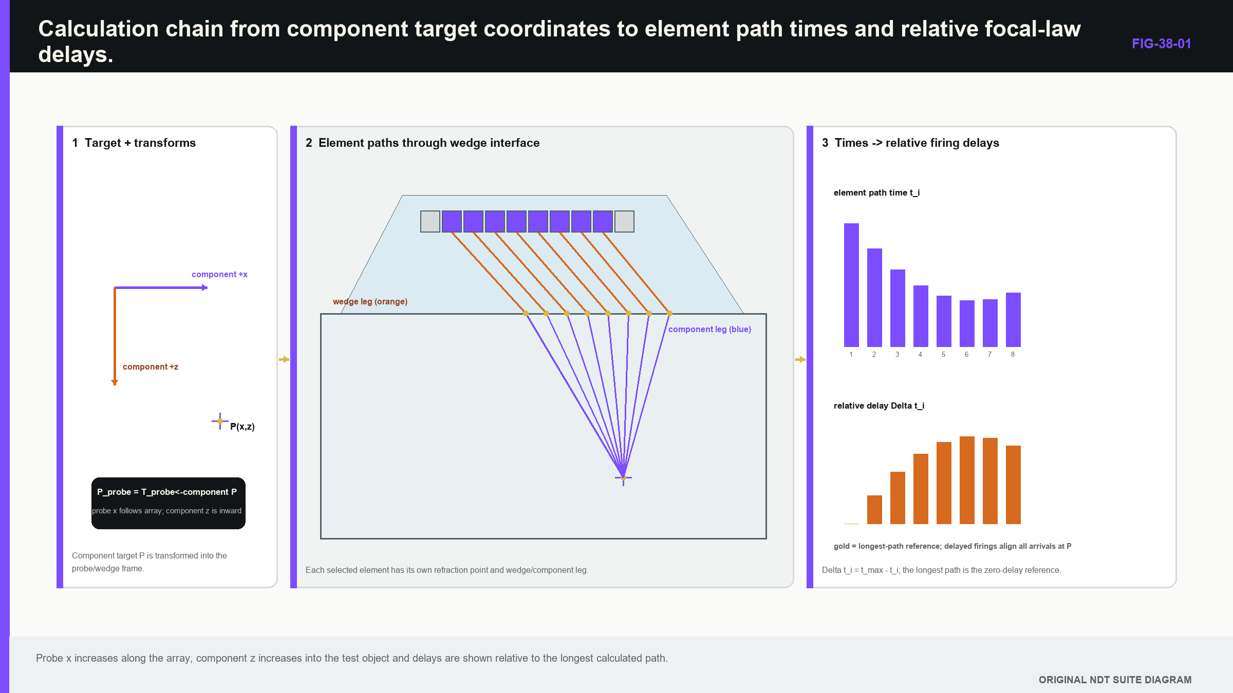
Notice that a delay value is the final output of geometry, velocity, path and timing conventions; it is not an independent property of the probe.
38.2 Homogeneous point focusing
For elements on a straight line in one isotropic material, each path length is the straight distance between the element centre and the chosen focus. The longest distance becomes the common reference. Divide every distance difference by wave speed to obtain relative delay.
| (38.1) Relative delays for a homogeneous point focus · EQ-38-01 Where: d_n = path from element n to the focus (m); x_n = element-centre coordinate (m); x_f = focus lateral coordinate (m); z_f = focus depth (m); d_max = largest active-element path (m); tau_n = relative delay applied to element n (s); c = represented wave speed (m/s) Model limits: homogeneous isotropic medium; elements lie on one line; focus lies in the model plane; hardware reproduces the calculated relative delays |
|---|
The equation supports delay sign, scale, smoothness and symmetry checks. It does not model wedge refraction, finite elements, material attenuation or the field width around the focus. Chapter 37 remains the next layer after path-time correctness.
| Worked example · Check the relative delay between neighbouring elements WE-38-01 Given: Element centres are at x = 0.0 mm and x = 0.6 mm. The intended homogeneous-material focus is at x = 10.0 mm, z = 30.0 mm. Use shear-wave speed c = 3,230 m/s. Find: The relative delay that aligns the shorter path with the longer path. Steps: Calculate both distances. d_0 = sqrt(10.0^2 + 30.0^2) = 31.6228 mm. d_1 = sqrt(9.4^2 + 30.0^2) = 31.4382 mm. The difference is 0.1846 mm = 0.1846 x 10^-3 m. Divide by velocity: tau = 0.1846 x 10^-3 m / 3,230 m/s = 57.2 ns. Answer: The element at x = 0.6 mm has the shorter path and receives about 57 ns delay relative to the element at x = 0.0 mm under this convention. Technical implication: The result checks sign and scale. It is not a production wedge law because the wedge leg, refraction, true element positions and hardware offsets are absent. Common mistake: Copying the 57 ns into a contact setup or reversing the sign because the reference-time convention was not written down. |
|---|
The value passes a physical sense check. A path difference below 0.2 mm at roughly 3.2 mm per microsecond should create a delay much smaller than 0.1 microsecond. A result of 57 microseconds would reveal a unit error immediately.
38.3 Ideal steering as a delay ramp
Steering a near-planar wavefront in one homogeneous medium requires a constant delay change between neighbouring elements. The path difference is element pitch multiplied by the sine of the steering angle, so the delay step is that path difference divided by wave speed.
| (38.2) Adjacent delay for ideal homogeneous steering · EQ-38-04 Where: Delta_tau = adjacent-element delay magnitude (s); p = element pitch (m); theta = steering angle from the aperture normal; c = represented wave speed (m/s) Model limits: uniform linear array; one homogeneous isotropic medium; planar steering objective; declared element numbering and delay-sign convention |
|---|
For p = 0.60 mm, theta = 30 degrees and c = 3,230 m/s, the delay magnitude is 0.60 x 10^-3 m x sin30 / 3,230 m/s = 92.9 ns. Reversing steering direction should reverse the ramp under a fixed numbering convention. A constant offset added to every element does not change relative steering, although it can affect absolute hardware timing and receive windows.
The equation is an excellent regression case because it has an expected straight-line delay plot. It does not establish refraction through a wedge, grating-lobe control or usable high-angle sensitivity.
38.4 Add the wedge and solve for the interface point
A contact PAUT path normally contains at least a wedge leg and a component leg. Each element may reach the target through a different point on the interface. That interface point is not generally the vertical projection of the element or target.
A solver is simply the calculation that finds the interface coordinate giving a physically valid travel path. For a planar isotropic boundary, the chosen path gives stationary travel time and satisfies Snell's law. A numerical root finder is often easier to implement and check than a closed-form expression, especially with curved surfaces.
| (38.3) Two-medium element-to-target travel time · EQ-38-02 Where: T_n = total time from element n to target (s); q = candidate interface coordinate (m); d_w,n = wedge-leg length from element n to q (m); c_w = wedge-mode speed (m/s); d_m = component-leg length from q to target (m); c_m = selected component-mode speed (m/s) Model limits: one declared transmitted mode in each leg; known interface geometry; representative velocities; geometrical path model without finite-beam or target-scattering terms |
|---|
The solver evaluates or minimises this time subject to physical boundaries. Its outputs should include interface point, incidence angle, refracted direction and travel time, not only the final delay. Those intermediate quantities reveal a solution that has crossed outside the wedge, selected the wrong surface or entered a mode beyond its physical range.
In anisotropic material, phase direction and group-energy direction can differ. Merely inserting a direction-dependent scalar velocity into isotropic Snell geometry can be inconsistent. The path solver must match the material model, or the law's apparent precision exceeds its physics.
38.5 Keep transmit, receive and electronics separate
Transmit delays choose when element pulses launch. Receive delays shift captured channels before summation. In a reciprocal static case with the same aperture and target, their geometric patterns can be related, but implementation may differ. Dynamic receive focusing can change aperture and delay with sample time or reconstructed depth.
A displayed transmit-focus label therefore does not prove the receive field. For multiple receive channels, a complete pulse-echo path uses transmit travel time plus receive travel time for each pair. Off-axis targets, different apertures and skewed geometry remove simple symmetry.
Electronic timing adds pulser, cable, channel, switching and digitiser offsets. A wedge-delay calibration may absorb several contributions into one number. That can be valid when the configuration is unchanged and the meaning is retained. Moving cables, substituting a probe or changing multiplexing can alter an offset while the software label stays the same.
Failure case: receive-time origin. A fixed transmit focus is correct, but targets appear progressively displaced after a firmware update. Raw transmit timing is unchanged. The receive schedule is indexed from a different sample-time origin. Checking only the exported transmit delays would miss the failure; reference targets at several depths reveal the depth-dependent shift.
38.6 Move between probe and component coordinates
The probe has its own frame, with element centres defined relative to an origin. The component has another frame tied to the scan datum and surface. A rigid transform rotates the probe frame and then translates it into component coordinates.
| (38.4) Rigid probe-to-component coordinate transformation · EQ-38-03 Where: r_component = point coordinates in the component frame (m); r_probe = point coordinates in the probe frame (m); R = orthonormal rotation matrix; t = translation vector from component origin to transformed probe origin (m) Model limits: rigid geometry; consistent units; declared right-handed frames; rotation and translation order fixed |
|---|
For an ideal rotation, the inverse is r_probe = R^T (r_component - t). The order matters. Rotating a point and then translating it is generally different from translating first and rotating about the component origin.
The probe origin, first-element centre, wedge index, tool centre and scan reference are distinct physical points. Calling each one “zero” creates silent offsets. A matrix array adds a second aperture coordinate; roof angle, curvature and skew add three-dimensional rotations. The familiar sector view remains only one slice.
Test transforms with non-collinear known points. One point checks a limited translation. Two points may check a scale and direction in a plane. Three-dimensional rotations need enough fiducials to expose all controlled axes. Fitting a transform to several points and reporting the same residuals is calibration; independent hold-out features provide stronger validation.
38.7 Path branches and solver continuity
Curved surfaces, multiple boundaries and mode conversions can allow more than one stationary path. Each physical solution is a path branch. As a target moves smoothly, the selected branch should normally move smoothly until a real boundary or mode transition occurs.
A numerical solver can jump between branches and produce discontinuous interface points or delays. Initialising from the previous solution encourages continuity but can also follow the wrong branch. Robust software enumerates plausible branches where needed, applies physical validity tests and records when a branch appears or disappears.
Plot interface coordinate, incidence angle, path time and delay against target position. A final law table can hide a branch jump that becomes an image seam or abrupt field change. Treat branch transitions as supported view boundaries, not as values to smooth away.
Evidence-boundary case. A generator returns a law for a target behind a geometric path limit by selecting its nearest feasible solution. The display still shows a sector, but the requested target was never supported. A released generator should reject or flag the request, and qualification should include targets near the limit to test this behaviour.
38.8 Tolerances and sensitivity
Every law uses measured or nominal inputs. Element pitch and position vary. Wedge angle, height and velocity vary with manufacture, temperature and wear. Component velocity can change by material, direction and mode. Probe placement and surface geometry differ from the model.
Sensitivity states how much an output changes when an input changes. Begin by perturbing one credible input and recalculating focus coordinate, arrival time and coherent response. Then examine interactions among influential inputs. A velocity increase and wedge-height change may cancel at one target while diverging at another.
A compact sensitivity matrix uses input variables as columns and outputs as rows. Large entries identify variables that need tighter measurement, control or verification. The matrix is configuration specific; transferring it to another wedge or material without recalculation is unsupported.
Parameter fitting creates correlation. A higher velocity and a larger electronic delay can match one narrow time range. Targets at several depths, angles and lateral positions provide different sensitivities and improve identifiability. Retain fitting objective, bounds, residuals and covariance when estimated inputs later support location uncertainty.
38.9 Delay quantisation and realised hardware
Hardware cannot reproduce infinitely precise delay. It rounds ideal values to a timing step. With nearest rounding, one channel's error is at most half a step, but the pattern across the aperture matters.
Phase error is 2 pi f delta_t. A 2 ns error is 3.6 degrees at 5 MHz and 7.2 degrees at 10 MHz. A broadband pulse sees a frequency-dependent error, not one fixed rotation. Random-like rounding tends to spread error; systematic stair-step patterns can create structured side response.
Simulate the realised law, including rounded delays, excluded channels and firmware constraints. Channel jitter, common clock phases and switching offsets can add further differences. Keep both ideal and realised tables. A law name does not reveal which one the instrument actually used.
Wedge temperature compensation is another realised function. Sensor location and response time matter. A surface reading taken after the scan may not represent wedge temperature during acquisition. If compensation affects accuracy, sensor identity, placement, timing, coefficient and algorithm version become controlled inputs.
38.10 Independent checks that challenge different failures
Minimum checks include element order, aperture extent, expected delay symmetry or monotonicity, steering sign, interface region, total path time and target coordinate. A delay-versus-element plot catches discontinuities. A reconstructed wavefront at two time steps catches sign reversal.
Agreement between two tools is not independent when both use the same geometry library, input file or export convention. Combine three forms of evidence where consequence requires it:
- an analytical homogeneous focus or steering ramp;
- a separately implemented wedge/path calculation; and
- a measured target with independently known coordinates.
The public scope of array vocabulary and PAUT documents can orient terminology and application boundaries, but it does not replace implementation evidence. [R042] [R046] Manufacturer material provides useful aperture and focal-law vocabulary while remaining system specific. [R014]
An inverse check starts with exported delays and determines the implied focus or wavefront. Fit a plane to a steering ramp or back-propagate emission times through the declared wedge. This can expose sign reversal, element-order swap or wrong velocity even if the intended target exists only inside a proprietary generator.
38.11 Export, reimport and change-impact cases
Digital errors can corrupt an otherwise correct law. Millimetres may become metres, element numbering may shift by one, sign may reverse or a file may be truncated. Export and reimport the law, compare identity and reconstruct its physical outputs. A checksum protects byte identity; the analytical and measured checks protect meaning.
Change-impact case. A firmware update preserves ideal law files but changes delay rounding from nearest to downward. Most central laws remain close; maximum-steering laws develop a structured residual across the aperture. The affected claims are not merely file compatibility. High-angle field shape, side structure and sensitivity need regression evidence using realised delays and worst-case targets.
If the system cannot export delays, compensating evidence must show geometry, timing and repeatability across saved setups and versions. A black-box law can still be controlled, but only by stronger external performance evidence and a narrower claim. [R014] [R016]
38.12 Release record and technical boundary
Every released law should resolve to element coordinates, probe and wedge identity, target or steering objective, velocities, interface geometry, coordinate frames, path branch, ideal delays, realised delays and software/firmware identity. Absolute and relative timing should be distinguished.
Failure cases should cover focus near the interface, maximum steering and skew, aperture clipping, invalid mode and a target beyond the path limit. The expected behaviour is documented rejection or a flagged reduced-support state. Silent nearest-solution behaviour is not an acceptable substitute.
The release question is whether another competent analyst can recreate the physical target, the path and the realised delays and then challenge them with independent evidence. Matching tables are insufficient if their coordinate convention is shared and wrong. [R014] [R016]
38.13 Evidence boundary for a family of laws
A sector or depth sequence contains many laws, but checking one central law does not automatically support the family. Select boundary cases from the mechanisms already identified: the largest steering magnitude, shallowest and deepest focus, aperture transition, array-end clipping and any path-branch transition. Add an interior case where competing input effects could cancel at an endpoint yet remain wrong between them.
Evidence should be output specific. A measured reflector at one coordinate can confirm arrival time and approximate location while providing little information about side structure. A field map challenges focus and unwanted response. A planar target challenges angular support. Hardware delay export challenges realisation but not acoustic coupling. The law family is released only for the outputs addressed by the combined set.
If a variable range is interpolated, verify that the path and delay behaviour remain continuous across it. A change of mode, branch or active-aperture rule breaks simple interpolation even when the software produces smoothly numbered laws. State such boundaries in the setup so an operator cannot extend the sequence merely by entering another angle or depth.
38.14 Substitution case: matching images from different delay tables
A setup is exported from one law generator and recreated on another platform. Both displays show a 40- to 70-degree sector focused at the same nominal depth, and the central reference reflector appears at the expected coordinate. The exported delay tables nevertheless differ by more than the receiving hardware step on several edge elements.
The first task is not to choose the better-looking sector. Rebuild the physical inputs: element coordinates and order, wedge geometry, velocities, probe origin, component frame, focus convention, transmit reference and receive rule. A reversed element order or different zero-delay convention can make tables appear different while producing equivalent relative timing. A different interface branch can produce similar central timing but diverge elsewhere.
Convert both files to one declared convention and compare relative delays, not only stored integers. Plot travel-time residual across the aperture for boundary and interior laws. Inspect where a constant offset, sign reversal, rounding pattern or element-dependent difference appears. A constant offset may preserve focusing but change absolute gate timing; a curved residual changes the wavefront.
Then compare realised outputs. Use known reflectors at shallow, deep and maximum-angle positions, plus a field or target scan sensitive to side structure. Retain raw timing before display transforms. If the platforms reconstruct coordinates differently, distinguish acquisition-law equivalence from display-coordinate equivalence.
Suppose the central and shallow laws agree, while the deep high-angle law shows a systematic edge-element residual caused by a different wedge-interface branch. The shared centre image did not prove the family. Release may remain possible for the continuous common range, while the branch transition is corrected, excluded or revalidated.
The law record therefore keeps ideal paths, normalised relative delays, hardware rounding and software identity. A checksum shows that each file is stable, while the independent calculation and target evidence show whether either file represents the intended acoustic path. [R014] [R016] [R042] [R046]
A receive-law comparison needs the same care. Dynamic receive focusing may store zones, update rules or derived parameters instead of one static table. Compare the realised receive delay at selected sample times across the aperture, then challenge those times with reflectors spanning the depth range. Identical transmit delays do not establish identical receive focusing.
Finally test reconstruction from retained raw data where the systems permit it. If the same waveforms produce different component coordinates, the discrepancy belongs to transformation or display processing rather than acoustic transmission. Separating those layers allows a limited transfer decision instead of rejecting or accepting the entire platform as one indivisible object.
Document any feature that cannot be exported or independently inspected. A proprietary receive rule may still be usable, but its evidence then relies more heavily on measured depth cases and controlled regression data.
In plain words
- A focal law stores timing instructions derived from a path and coordinate model; it does not store a beam by itself.
- Shorter paths are delayed to meet a common arrival time under the longest-path convention.
- Wedge laws need a solver that finds a physically valid interface point for every element.
- Transmit timing, receive timing and electronic offsets must remain distinct.
- Probe, wedge, scanner and component origins are different points joined by declared transforms.
- Tolerance and delay rounding matter only through the change they cause in field, time or coordinate outputs.
- Independent checks must challenge different failure modes rather than repeat one implementation.
- Released records retain both the ideal law and the timing actually realised by hardware.
Formal synthesis
Focal-law control connects element coordinates and component targets through a travel-time forward model. Homogeneous point focusing and steering provide analytical checks; contact PAUT requires interface solutions and explicit coordinate transforms. Sensitivity, branch continuity, delay quantisation, electronics and software identity determine whether ideal delays survive as a reproducible physical field. Level 3 release therefore verifies calculation, validates target behaviour and preserves the evidence boundary of each law family.
Key terms
- Reference time: common arrival time used to form relative delays.
- Solver: method that finds a path satisfying the model and boundary conditions.
- Path branch: one candidate physical solution among possible interface paths.
- Rigid transform: rotation and translation joining probe and component frames.
- Sensitivity matrix: local map from input changes to output changes.
- Delay quantisation: hardware rounding of continuous ideal delays.
- Realised law: active channels and delays actually implemented by the system.
Key relationships
- EQ-38-01 converts homogeneous element-to-focus path differences into relative delays.
- EQ-38-04 gives the constant adjacent delay magnitude for ideal planar steering.
- EQ-38-02 adds wedge and component travel times through a candidate interface point.
- EQ-38-03 rotates and translates probe coordinates into the component frame.
Common mix-ups
- Relative delay equality is not absolute timing equality.
- A displayed focus coordinate is not proof that the realised field peaks there.
- Probe origin, wedge index and first-element centre are not interchangeable.
- Two agreeing law generators are not independent if they share inputs or code.
- Checksum identity proves bytes are unchanged; it does not prove the law is physically correct.
Bridge to Chapter 39
Chapter 38 controlled phase timing at the chosen element positions. Chapter 39 asks whether those positions sample the desired aperture finely enough. It explains how pitch, wavelength, steering, element width and sparse selection can create unwanted beams even when every focal delay is mathematically correct.
Sources and further study
- [R014]
- [R016]
- [R042]
- [R046]
Study and revision only. This is not an approved inspection procedure, acceptance criterion or qualification.