
CHAPTER 49 · FMC / TFM / PCI Level 2
Building a TFM Image One Pixel at a Time
In this chapter · 21 sections
Why this matters
A TFM image often looks like a cross-section of the component, but the probe never photographs that cross-section; every pixel is calculated from stored A-scans and a travel-time model. The processor predicts when a signal from that location would arrive in each transmitter-receiver trace, selects the corresponding samples and combines them. Understanding one pixel makes the whole image less mysterious. It also explains why wrong velocity, surface geometry, path choice or timing can create a sharp response at an incorrect coordinate.
What you already need
- The Chapter 47 matrix-cell picture and signed RF waveform.
- The Chapter 48 requirement for complete, unclipped and positioned source data.
- Basic distance, velocity and time relationships.
- The PAUT idea that delayed waveforms reinforce when aligned.
- Simple coordinate and right-triangle calculations.
What you will learn
- Define a reconstruction region and one candidate pixel.
- Calculate a direct transmitter-to-pixel-to-receiver travel time.
- Select and combine samples for two simple pixels.
- Explain why interpolation is needed between stored sample times.
- Recognise the extra legs introduced by wedges, reflections and mode conversion.
- Distinguish pixel spacing from the physical point-spread response.
Words you will meet
- Region of interest: the declared coordinate area in which pixels are calculated.
- Travel-time model: the geometry and velocities used to predict an arrival for each pair.
- Delay and sum: alignment of pair contributions by predicted time followed by combination.
- Interpolation: estimation of a waveform value between stored sample times.
- Weight: a declared factor that changes one pair contribution before combination.
- Point-spread response: the finite image shape produced by a small target.
- Aperture support: the useful transmitter-receiver geometry contributing to a pixel.
49.1 Start with one known point
Place a small reflector at a known coordinate beneath an array. Choose transmitter element 4 and receiver element 17. Sound travels from element 4 to the reflector and then from the reflector to element 17. The total travel time is the first distance divided by the selected wave speed plus the second distance divided by its selected speed.
The pair A-scan contains many sample values through time; the reflector is not stored with a pixel label. The processor uses the predicted pair time as an address into the waveform; a different candidate point gives a different time. A different transmitter-receiver pair gives another time for the original point. TFM repeats this address-and-combine operation across a region of interest (ROI). The method is therefore easier to understand in the order one point, one pair, many pairs, two points, then the full grid. Open technical accounts describe TFM as a model-based delay-and-sum reconstruction from elementary matrix signals rather than a direct image measurement. [R017] [R047]
49.2 Draw both legs before calculating
The following figure shows the minimum direct-path picture; the transmit and receive elements sit at known coordinates. The candidate pixel sits inside the component; one leg joins the transmitter to the pixel and the other joins the pixel to the receiver.
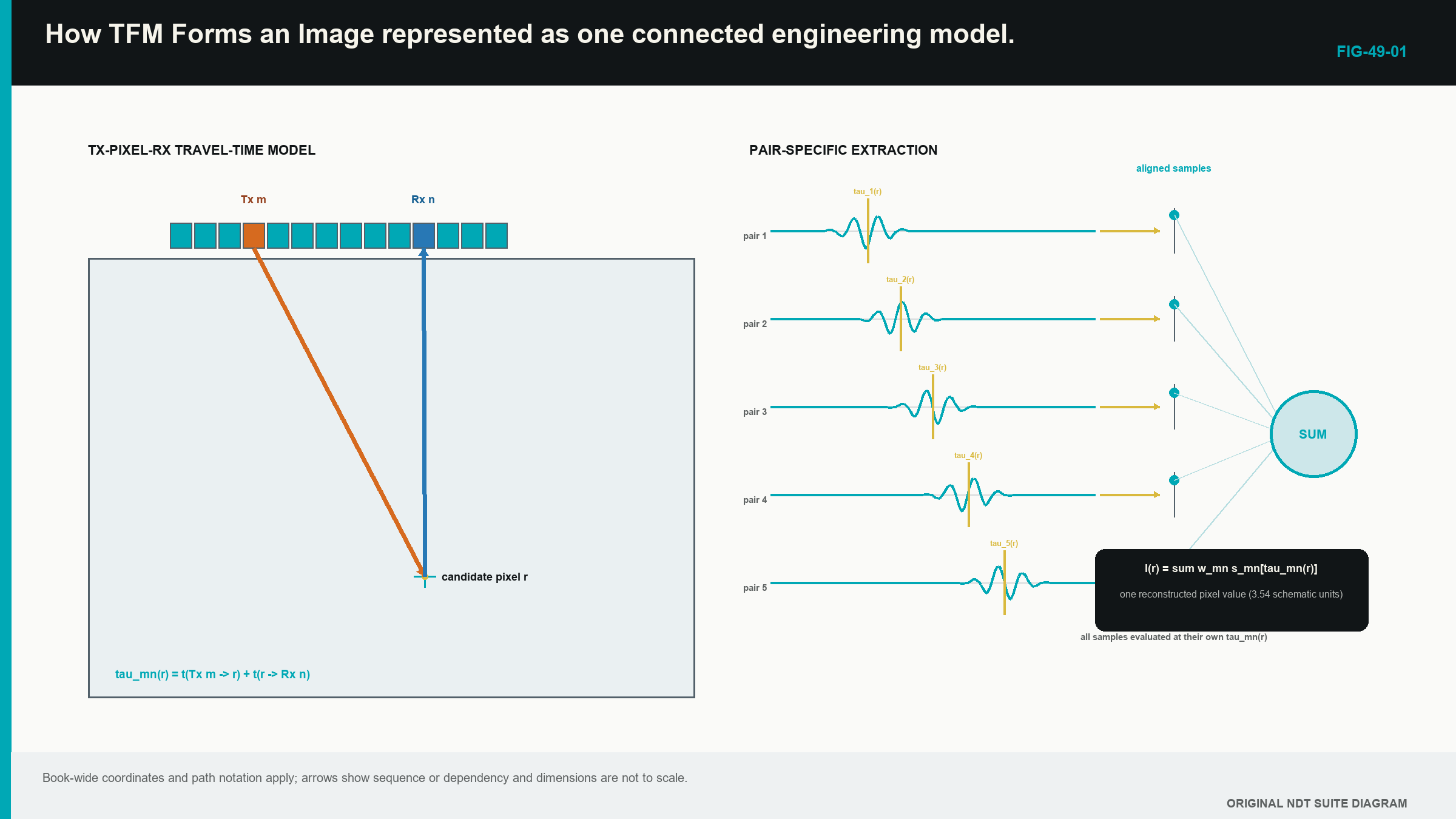
The two-leg drawing prevents a familiar mistake; most off-diagonal FMC cells are pitch-catch records, so pulse-echo distance divided by two is not the general route. Each leg has its own length; if transmit and receive modes differ, each leg also has its own speed.
The predicted time is only an address; it does not prove the candidate point contains a reflector. The test comes from whether many physically useful pair traces contain consistent signal at their own predicted times.
49.3 Define the grid in component coordinates
The ROI has an origin, width, depth range and pixel increments; it uses the same component coordinate system as the probe position and encoded scan. The technique also needs element locations, array orientation, wedge or surface geometry and the positive coordinate directions.
The box does not prove acoustic coverage. Software can calculate pixels outside usable directivity, penetration or path support. Expanding the ROI creates more calculations, not more transmitted sound. Chapter 51 separates the numerical grid from physical coverage.
Registration errors change every pair address; an incorrect encoder offset moves the array model relative to the component. A wrong wedge height changes interface travel time; a flat surface used in place of real curvature changes entry points and refraction. These are not screen-layout differences; they determine which samples are visited.
Keep the first exercise simple. Use a homogeneous block, a direct path, one known velocity and element coordinates on a flat surface. Complicated interfaces become easier after the learner can explain this base case without software.
49.4 Calculate a direct pair time
For a candidate position r, let transmitter position be e_i and receiver position be e_j. In a homogeneous region, the processor calculates the distance from transmitter to pixel and the distance from pixel to receiver. Each is divided by the speed assigned to that leg.
| (49.1) Direct two-leg TFM delay for a selected mode pair · EQ-49-01 Where: tau_ij^(m-n)(r) = predicted time for transmitter i, receiver j and mode pair m-n at pixel position r (s); r = pixel position (m); e_i = transmitter position (m); e_j = receiver position (m); c_m = transmit-leg mode speed (m/s); c_n = receive-leg mode speed (m/s); ||.|| = straight-line distance Model limits: direct straight legs in a homogeneous isotropic region, a declared time origin and no intervening reflection or conversion |
|---|
Use one numeric point. A transmitter at x = 0 mm, receiver at x = 10 mm and candidate at x = 6 mm, z = 20 mm give transmit distance sqrt(6^2 + 20^2) = 20.88 mm and receive distance sqrt(4^2 + 20^2) = 20.40 mm. At 5.90 mm/microsecond, the total time is (20.88 + 20.40)/5.90 = 7.00 microseconds.
The units provide a check. Millimetres divided by millimetres per microsecond give microseconds. A result near 70 microseconds would be a decimal error for this small block, while 0.70 microseconds would imply an unrealistically short route.
| Worked example · A symmetric direct-path pixel WE-49-01 Given: A transmitter and receiver are each 10 mm horizontally from a candidate pixel at 20 mm depth. Both direct legs use 5,900 m/s. Find: The predicted two-leg travel time. Steps: Each leg is sqrt((10 mm)^2 + (20 mm)^2) = 22.36 mm. Total distance is 44.72 mm = 0.04472 m. Divide by speed: 0.04472 m / 5,900 m/s = 7.58 x 10^-6 s. Answer: The reconstruction visits that pair trace near 7.58 microseconds for the candidate pixel. What it means in practice: A wrong element position or velocity moves the visited sample and can shift or defocus the reconstructed response. Common mistake: Applying distance = velocity x time / 2 to an off-diagonal pair ignores that the transmit and receive legs begin at different positions. |
|---|
49.5 Build two pixels with four traces
Take four healthy pair A-scans from a small teaching matrix. For Pixel A at the known reflector, the predicted times visit signed RF values of +0.70, +0.82, +0.61 and +0.75 in the same chosen units. Their signs and cycle positions agree, so the simple sum is +2.88.
Pixel B lies nearby in background material; its four predicted times visit +0.50, -0.42, +0.21 and -0.30. The signs partly cancel, giving -0.01; the traces themselves have not changed. The two pixels ask for different times from those traces.
This tiny example explains how a bright pixel can be formed even when no single A-scan contains an enormous obvious peak. Many modest, consistently timed contributions reinforce; it also explains why one unusually large trace can dominate an unsupported image value. A robust audit checks whether the result is distributed across a useful aperture.
Real TFM uses more pairs and normally evaluates waveform values with interpolation; the four-trace sum is a teaching model, not a vendor algorithm. It establishes the physical sequence before notation.
49.6 Express delay and sum formally
After the hand-built pixels, the general relationship becomes readable. At each pixel, the processor visits the predicted time in every included trace, applies its declared weight and adds the contributions.
| (49.2) Weighted delay-and-sum reconstruction · EQ-49-02 Where: I_P(r) = reconstructed signed value for selected path P at pixel position r (weighted voltage or digitiser units unless the implementation defines another scale); i = transmitter index; j = receiver index; w_ij,P(r) = declared pair weight (dimensionless unless otherwise stated); s_ij(t) = elementary RF waveform value at time t (voltage or digitiser units); tau_ij,P(r) = predicted pair time (s) Model limits: pair set, polarity, time origin, interpolation, weights and acoustic path are declared consistently |
|---|
The weight can represent aperture selection, apodisation, directivity or another documented correction; a weight of zero excludes the pair. Weighting can reduce some artefacts or compensate a modelled effect, but it also changes the technique; a clean result is not proof that the chosen weights are valid.
Some implementations sum real RF first and form an envelope later. Others use analytic signals or frequency-domain calculations. The equation is a vendor-neutral reference model. The software name and version must state the actual processing route.
TFM in ordinary one-element-at-a-time FMC does not transmit one physical beam focused at each pixel. The focusing is synthesised after capture. The wording total focusing describes repeated calculated alignment, not uniform resolution or sensitivity throughout the ROI.
49.7 Add wedges, reflections and conversions one leg at a time
An angle-beam setup adds a wedge leg and an interface crossing. The path from one element to one pixel is no longer a single straight segment at one speed. Refraction can place a different entry point for every element-pixel combination.
A reflected view adds a known surface and a reflection point. A mode-converted view assigns different speeds to legs before and after conversion. The general time is the sum of each declared leg length divided by the speed of its medium and mode.
| (49.3) General piecewise travel-time model · EQ-49-03 Where: tau_ij,P(r) = predicted transmitter-i-to-pixel-r-to-receiver-j time for selected path P (s); q = path-leg index; l_q = length of leg q (m); c_q = speed assigned to that leg (m/s); P_Tx = ordered transmit-side leg set; P_Rx = ordered receive-side leg set Model limits: every interface point, reflection, conversion and mode in the selected stationary path is physically admissible |
|---|
The equation supplies travel time, not sensitivity. A mathematically possible path may transmit very little energy because of incidence angle, directivity, attenuation, path length or reflector orientation. Chapter 50 develops that distinction with a small set of direct, reflected and mode-converted views.
49.8 Interpolate between stored samples
Suppose samples are stored every 0.02 microseconds, while a predicted time is 7.01 microseconds. The required time lies halfway between stored values. Nearest-sample selection chooses one neighbour. Linear interpolation estimates between them. Spline, sinc and frequency-domain methods use other assumptions.
Interpolation can make peak position and amplitude more stable, but it does not create independent acoustic bandwidth. If the waveform was sampled poorly or filtered before storage, a smooth estimate remains based on limited information. The actual method should be controlled when it affects qualification or comparison.
Processing continues after the signed sum. An RF reconstruction retains positive and negative cycles. An envelope displays magnitude around the oscillation. Rectification changes how signs appear. Normalisation can make weak and strong images reach the same displayed maximum. A colour scale can improve visibility without improving source signal-to-noise ratio.
When comparing reconstructions, record the signal domain, scaling and post-processing. Two images with identical colours can represent very different physical quantities and absolute response levels.
49.9 Pixel spacing is not the point response
A very small reflector does not normally become one square pixel. It produces a finite point-spread response with depth width, lateral width and side structure. Frequency, bandwidth, aperture, element pitch, directivity, path geometry, target type, interpolation and weighting all contribute.
Smaller pixels sample that shape more finely. They may give a smoother picture and reduce the chance that the peak sits between grid points. They do not narrow the physical response by themselves. A side-drilled hole also contributes its own extended scattering behaviour and should not be described as a universal point.
Apparent image width is therefore not automatically reflector width. Two reflectors are resolved only when their overlapping responses remain distinguishable under a declared criterion. The criterion and performance vary across the region and across different views.
Chapter 51 reconstructs the same source dataset with different grids, apertures, filters and display settings so the learner can see which changes affect numerical appearance and which affect actual demonstrated performance.
49.10 Trace one feature back to its contributors
Begin with dataset and reconstruction identity. Draw the selected path. Confirm that the feature lies within the demonstrated ROI and the required time range. Open representative diagonal, near and wide pair traces. Compare their observed signal packets with the pixel times used by the reconstruction.
After applying the same delays, look for residual timing patterns across transmitter and receiver positions. A steady slope can indicate velocity, geometry or timing mismatch even when the total sum remains bright. Check that support is distributed across the expected aperture rather than dominated by one channel.
Change one model input at a time on a working copy. A corrected velocity should alter position and focus in a predictable way. A different physical path should have its own travel-time and geometry argument. Compare a materially different view, a repeat position or conventional evidence where available.
An audit display that exposes pair identity, predicted time, interpolation and selected value is valuable because it joins the image back to its source. Removing one dominant unexplained pair is a sensitivity check, not an authorised production repair. Formal residual and implementation analysis continues in Chapters 56 to 58. [R017]
49.11 The Level 2 boundary
The learner should be able to draw a direct path, calculate a pair time, explain sample selection, identify the main assumptions and challenge a feature with source traces. The learner is not required to derive Green functions, implement a ray solver, design an interpolation kernel or prove a commercial functional.
Chapter 56 introduces imaging functionals at Level 3. Chapter 57 treats planar, curved, layered and anisotropic path solvers. Chapter 58 develops numerical error and determinism. Chapters 69 and 72 provide the engineering depth for signal estimation and advanced image formation.
In plain words
- A TFM pixel is calculated from stored pair A-scans and a travel-time model.
- Each transmitter-receiver pair has its own predicted time for the same pixel.
- A different pixel visits different times in the same source traces.
- Delay alignment allows physically consistent waveform contributions to reinforce.
- Wedges, reflections and conversions add declared path legs and speeds.
- Interpolation estimates between stored samples but does not create new bandwidth.
- Tiny pixels sample an image more densely; they do not guarantee finer physical resolution.
- A defensible feature can be traced back to plausible paths and distributed waveform support.
Key terms
- ROI: component-coordinate region in which pixels are calculated.
- Travel-time model: declared geometry, interfaces, modes and speeds used to address samples.
- Delay and sum: pair-specific timing followed by coherent combination.
- Interpolation: estimate of a value at a time between stored samples.
- Weight: declared factor applied to a pair contribution.
- Point-spread response: finite image shape created by a small target.
- Aperture support: useful transmitter-receiver distribution behind a pixel.
Key relationships
- tau = transmit-leg time + receive-leg time: one pixel address includes both sides of the pair route.
- I_P(r) = sum of weighted pair samples: a TFM pixel combines values selected at pair-specific predicted times.
- piecewise time = sum of leg length/speed: wedges, reflections and conversions are added leg by leg.
- pixel spacing != physical resolution: numerical sampling and acoustic response are related but distinct.
Common mix-ups
- A pixel is calculated evidence, not a direct photograph of material.
- Pulse-echo divide-by-two is not the general formula for an off-diagonal pair.
- A physically possible travel time does not prove useful sensitivity.
- Interpolation smoothness does not equal new acoustic information.
- Image width does not automatically equal discontinuity width.
Bridge to Chapter 50
Chapter 49 used one direct path to make the pixel calculation clear. Chapter 50 expands the path vocabulary carefully. It introduces direct longitudinal and shear views first, then one reflected and one mode-converted route before showing why multiple valid-looking paths can compete.
Sources and further study
- [R017]
- [R047]
Study and revision only. This is not an approved inspection procedure, acceptance criterion or qualification.