Recognising When the PAUT System Has Changed

Why this matters

An array can lose one element, a wedge can wear and an encoder can slip while the sector image still looks believable. Performance checks compare the current system with an accepted baseline so those changes are noticed before they become unexplained data errors. This chapter begins with three visible symptoms: a weak patch in an element map, a shifted reference echo and a stretched encoded strip. It then connects each symptom to the part of the measurement it can affect. The aim is diagnosis and evidence, not a ritual checklist.

What you already need

• Calibration establishes separate timing, sensitivity and position relationships.
• A focal law combines several transmit and receive elements.
• A failed element can change the field without removing the whole image.
• Echo position and echo amplitude are different measurements.
• Encoded position has scale, polarity, zero and offset.

What you will learn

• Explain the difference between a baseline, a routine check and requalification.
• Read a basic healthy, weak or dead element response map.
• Connect reference-echo changes to timing, gain, coupling or component causes.
• Recognise encoder scale, direction and continuity symptoms.
• Use amplitude change in decibels to compare a current response with baseline.
• State which data outputs may be affected when a check fails.

Words you will meet

• Baseline: an accepted reference state used for later comparison.
• Routine check: a repeat observation intended to reveal change from baseline.
• Dead element: an element with no usable response under the stated check.
• Weak element: an element with materially reduced response under comparable conditions.
• Linearity: agreement between controlled input change and displayed change.
• Drift: gradual or sudden movement away from an accepted value.
• Requalification: broader evidence required after significant failure, repair or change.

34.1 Three symptoms on the screen

First, imagine an element-response map. Most element positions produce a similar band, but one produces no response and its neighbour is much lower. The sector view still contains echoes because surrounding elements remain active. The beam formed by any aperture containing those elements, however, can change in sensitivity and shape.

Second, imagine a reference echo that was at the correct path yesterday but is shifted today. Its amplitude is similar. That pattern points toward timing, velocity, delay or echo-selection change rather than a simple gain change. If spacing between several known echoes also changes, time-base scale or velocity becomes more likely than one fixed zero shift.

Third, imagine a known 500 mm scanner travel displayed as 525 mm. The ultrasonic echo times remain stable. That pattern points toward encoder scale or wheel mechanics. If the length is correct but direction is reversed, polarity is involved. If small sections repeat or disappear, continuity or overspeed may be involved.

Symptoms do not identify a cause by themselves, but they show which measurement function changed and which comparisons can separate plausible causes.

34.2 Baseline, routine check and requalification

An initial characterisation or accepted setup establishes baseline observations. These might include element response, reference amplitude, echo position, encoder travel or selected system behaviour. The baseline records the configuration and conditions needed to reproduce the comparison.

A routine check samples selected functions to reveal change and is narrower than full calibration or qualification. Passing one reference-amplitude check does not prove encoder direction, element health or beam coverage.

A significant failure, repair, substitution or software change may require recalibration or broader requalification. The response depends on the affected function and the controlling quality system. Repeating one convenient check is not enough when the changed item influences several parts of the measurement.

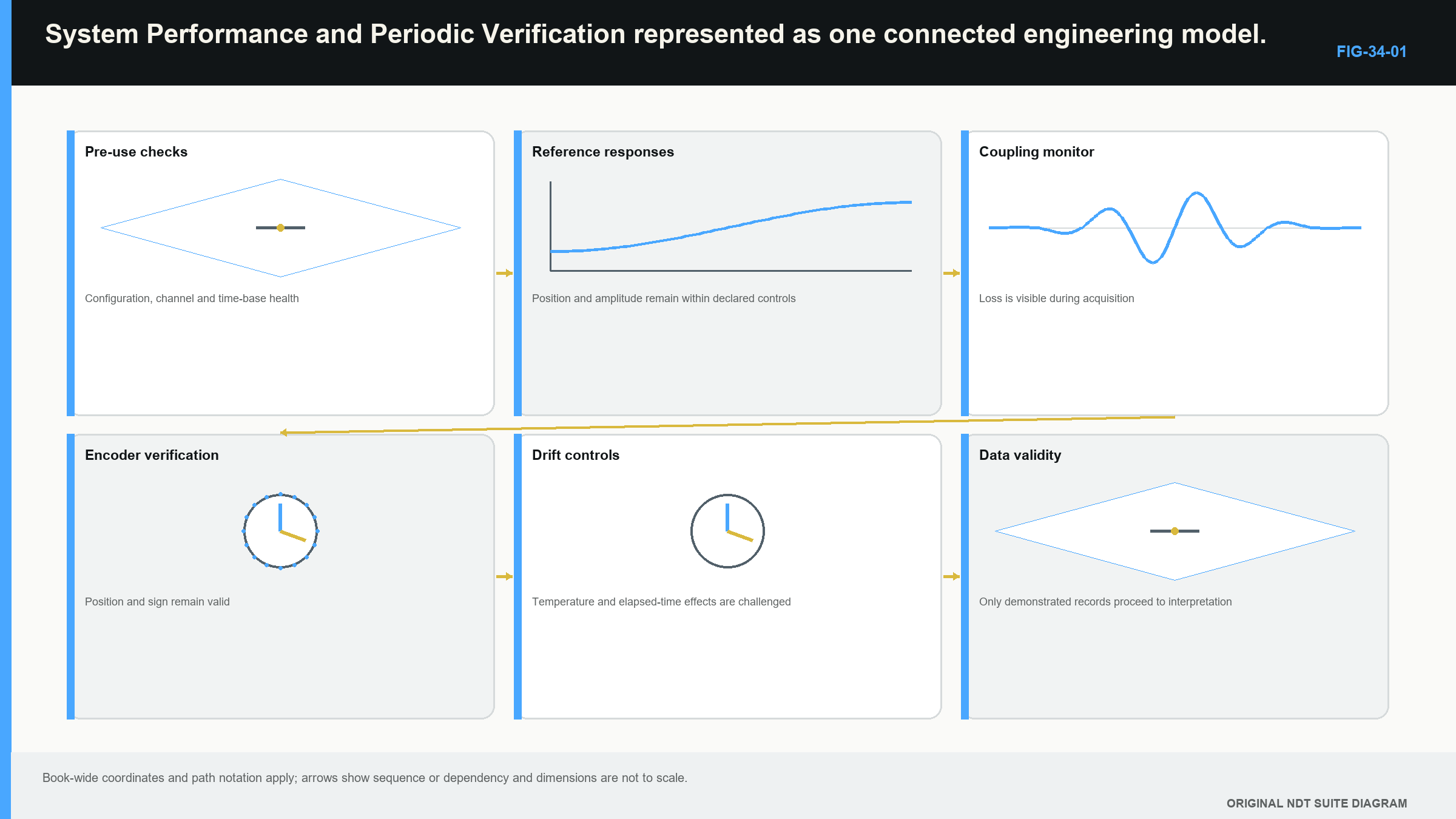
The check plan connects each observation with its reason, setup, expected result, tolerance source, timing and response to failure. Standards and guides define control layers and public scopes, but this study chapter does not invent their protected procedures, values or intervals. [R043] [R044] [R045] [R049]

The following figure links common checks to the evidence they protect. Follow each arrow to see why one green result cannot stand in for every other function.

34.3 Reference amplitude and position

Use the accepted setup and a known reference target. Reproduce probe position, coupling and relevant instrument settings. Compare both amplitude and echo position across the nominated laws or apertures.

A lower amplitude can come from changed gain, filter or pulser settings, weak coupling, wedge wear, cable damage, probe change, target positioning or element condition. A common amplitude fall across many laws suggests a common path or setting. A local fall over apertures sharing particular elements suggests a channel or element problem.

A common timing shift can come from delay, wedge temperature, probe seating or zero change. A changing error across path can point toward velocity or time-base scale. A shift only on some laws can point toward law-specific timing, element order or target interaction.

Record the expected and observed amplitude and position separately. A response can remain at the right time while losing amplitude, or remain at the same amplitude while moving. Combining both into one pass label destroys useful diagnostic information.

34.4 Healthy, weak, dead and misconnected elements

An element check aims to compare individual elements or small controlled apertures under similar acoustic conditions. A stable target or fixture should illuminate the element positions comparably. The result can be shown as a plot or map against element number.

A healthy element follows the accepted response pattern within the stated comparison. A weak element produces a materially lower response. A dead element produces no usable response. A misconnected or misordered channel can produce a response at the wrong element address.

Check suspicious results after restoring coupling and connectors. A target that is too small or poorly aligned can make outer elements look weak. Cable or adaptor faults can imitate probe damage. Automatic normalisation can hide raw differences. Systematic substitution helps separate probe, cable and instrument paths.

Clusters matter. One failed element may have a modest effect on a large aperture. Several adjacent failures create a larger inactive region and can alter steering, focus and side structure more strongly. There is no universal allowable number that applies to every aperture and law group; consequence depends on location, adjacency and technique.

The map also needs correct element order because every channel showing an echo does not prove correct mapping. A reversed or shuffled pattern can steer or position the field incorrectly while maintaining overall signal activity.

34.5 Encoder scale, direction and data continuity

Move the scanner over a known distance under representative contact. Compare physical and displayed travel, verify positive direction and inspect return or reverse behaviour when relevant. Then review a short encoded acquisition for regular positions and complete data.

Scale error stretches or compresses indication length and component coordinates. Polarity error mirrors the scan direction. Slip creates non-uniform local error. Backlash appears around reversals. Overspeed can cause gaps, irregular spacing or incomplete law sets.

Check every used axis. A correct scan encoder does not prove the index axis. A perfect encoder trace does not prove that the probe remained aligned or coupled. The wheel, mount, guide and surface are part of the check condition.

When a corrected view appears displaced but raw echo time remains sensible, compare the position chain: encoder count, scale, zero, sign, probe reference and offset. This avoids recalibrating ultrasonic time to solve a mechanical position fault.

34.6 Vertical and horizontal linearity in plain language

Vertical linearity concerns response height. Under reproduced conditions, a controlled change in gain or attenuation should produce the expected change in unsaturated amplitude over the used range. Begin with a stable echo away from clipping and the noise floor. Keep pulser, filter, rectification, averaging and gate behaviour fixed.

Approximately 6 dB corresponds to a factor of two in voltage amplitude under the same impedance. This is an amplitude relationship, not a power statement. If a displayed response does not follow controlled steps, amplitude evaluation may be affected.

Horizontal linearity concerns time or path position. Known echo intervals across the used range should be represented consistently. A fixed delay shifts all echoes together. A scale error changes the separation between echoes. Wrong velocity can also change displayed path while the instrument time base itself remains stable.

These checks answer measurement-function questions, but they do not show whether a particular beam reaches a natural discontinuity or whether inspection coverage is sufficient.

34.7 Compare current amplitude with baseline in decibels

When the same reflector is measured under reproduced unsaturated conditions, the change in linear amplitude can be expressed in decibels. The physical meaning comes first: the ratio compares current response with baseline. A negative result means the current response is lower.

34.8 Match a failed function to affected data

A failed check creates a data-validity question. Preserve the failed result and identify when the system was last known to be acceptable. Then separate which outputs depend on the failed function.

A timing fault can invalidate sound path, depth and corrected position while leaving some qualitative response evidence. An amplitude drift can affect threshold and amplitude-based evaluation while preserving encoded length. A reversed encoder can invalidate scan coordinates while leaving A-scan time relationships intact. Failed elements can affect sensitivity, focus and lobe behaviour for every aperture that uses them.

The affected data interval begins after the last acceptable evidence, not automatically at the moment the failure was noticed. Component substitution, impact, temperature change or setup editing can help bound the interval. The authorised quality process determines reacquisition or disposition.

Do not adjust the setup until the reference response passes and then discard the failed observation. The failure pattern is evidence needed to understand earlier data and prevent recurrence.

Walk through four failed-check patterns

Pattern 1: every law loses about the same amplitude. Begin with common conditions. Reproduce coupling and target position, then check gain, filters, cable, wedge contact and temperature. One dead element is less likely to lower every aperture equally than a common path or setting. If timing remains correct, location evidence may survive while amplitude-based evaluation needs review.

Pattern 2: only apertures containing elements 18 and 19 lose response. Compare the element map with the law table. Restore connectors and coupling, then repeat the element check. If the low response follows those physical channels across comparable apertures, probe, cable or channel condition becomes more plausible. Laws that do not use them may remain unaffected, but the complete technique still needs an authorised impact decision.

Pattern 3: every known echo moves by nearly the same time amount. A common delay, wedge seating or zero change is more plausible than material velocity when the intervals between echoes remain stable. Check wedge condition, temperature, probe mounting and timing settings. Correcting one common offset should not be used to hide an unexplained physical change.

Pattern 4: the first half of an encoded strip has the right scale and the second half is compressed. A single encoder scale value cannot explain a local change by itself. Wheel slip, lifting, contamination, guide movement or missed counts are more plausible. Compare raw positions with the physical path and reacquire the affected region after restoring the mechanism.

These patterns show why diagnosis begins with the shape of the change. Common, local, fixed and progressive errors point toward different parts of the measurement chain.

Separate a harmless display change from a measurement change

Not every visible change means the acquired data changed. A new colour palette can make the sector brighter while the underlying amplitudes remain identical. Changed interpolation can smooth an encoder strip without adding positions. A different corrected geometry can move pixels while raw A-scan times stay fixed.

Compare raw waveform values, setup identity and stored positions before treating a visual difference as system drift. Conversely, do not dismiss a stable-looking image when the element map or reference timing has changed. PAUT displays are very good at looking calm during technical mischief.

The check evidence should identify which layer changed: acquisition, processing, correction or display. Only changes that affect the measurement relationship need technical disposition, but every unexplained difference deserves the correct layer before it is accepted as harmless.

Use substitutions to narrow the cause

When allowed by the controlled diagnostic process, change one component at a time. Reconnect the cable, then repeat. Substitute a known compatible cable, then repeat. Fit another identified probe or wedge and establish the relationships it requires before comparing.

If the abnormal pattern follows the probe, the probe becomes more likely. If it remains with one instrument connector, the electronic path becomes more likely. If it disappears when coupling is stabilised, the original acoustic contact was involved. Each substitution changes the evidence; it does not grant permission to use the replacement without its required calibration.

Check the consequence at representative laws

After identifying a changed element or common response, inspect focal laws that use the affected path differently. Compare an aperture that excludes the element, one that places it near the edge and one that places it near the centre. The response can reveal whether the effect is local or distributed through the group.

Repeat the comparison at a near and far reference path when the technique depends on both. A change that looks small at one easy target can become important after steering, attenuation or distance correction. The aim is not to prove the whole technique during a routine check. It is to avoid assuming that one central law describes every affected beam condition.

Record the representative laws chosen and why. That note lets the responsible reviewer judge whether the check was sensitive to the failure mode that actually occurred.

The check should be reproducible by another competent person using the same identified reference. If its result depends on a hidden cursor choice, undocumented peak-hold state or one operator's pressure, the variation cannot be separated from real system change. Reproducibility begins with visible settings and a stable physical comparison.

Repeatability within one session is only the first test. A useful baseline can be reproduced after the equipment is disconnected and reassembled under the stated conditions. Reassembly challenges connectors, probe seating, wedge fit and setup identity. If the result cannot be recreated, later drift cannot be distinguished confidently from ordinary setup variation.

34.9 A useful check record

A useful record connects the comparison to one identified configuration. It includes job and component; date and examiner; instrument, software, probe, wedge, cable, scanner and encoder; setup and group identity; reference block and target; relevant conditions; expected value and controlled tolerance; observed value; evidence file; result; action and repeat result.

The record should preserve the numerical observation, not only “pass.” Trends and failure discrimination are developed later, but even Level 2 comparisons become more useful when the raw response, element plot or encoder trace is retained.

Check frequency comes from the governing requirement and technical risk. This chapter deliberately supplies no universal interval or tolerance. The learning objective is to understand why the check exists and what a change can affect.

Step up: spectrum and trend diagnosis

Centre-frequency and bandwidth checks use an RF waveform and a controlled Fourier-transform method. Long-term trending can separate gradual wear from sudden configuration change. Fault injection can test whether a check detects the failure it claims to control. These topics move to the Level 3 and engineering chapters because they require sampling, spectral-window and diagnostic-design depth. They are not assessment dependencies here.

In plain words

• A baseline is an accepted comparison state; a routine check samples selected functions.
• A plausible image can survive a weak or dead element.
• Amplitude and timing changes should be recorded separately.
• Encoder checks cover scale, direction and continuity, not acoustic geometry.
• Vertical linearity concerns controlled response-height change.
• Horizontal linearity concerns time or path representation.
• A failed function can invalidate some outputs while leaving others usable.
• Failed evidence should be preserved so earlier data can be assessed.

Key terms

Baseline; routine check; dead element; weak element; channel order; vertical linearity; horizontal linearity; drift; data-validity interval; requalification.

Key relationships

• current response / baseline response -> amplitude change in dB;
• common amplitude loss -> investigate common coupling or system path;
• law- or aperture-specific loss -> investigate elements, channels and geometry;
• fixed echo shift -> investigate delay or zero;
• changing echo interval error -> investigate scale or velocity;
• failed function -> identify dependent measurements and affected data interval.

Common mix-ups

• A routine check is not full application calibration.
• A live sector image does not prove every element is healthy.
• A timing shift is not repaired by gain adjustment.
• High encoder count density does not prevent wheel slip.
• Passing one check does not validate unrelated measurement functions.

Bridge to Chapter 35

The array system can now be built, calibrated and checked. Chapter 35 starts from the component and target rather than the equipment, then develops a coverage argument that connects access, probe position, beam regions and known limitations.

Sources and further study

• [R043]
• [R044]
• [R045]
• [R049]