
CHAPTER 39 · Phased Array Ultrasonics Level 3
Element Spacing, Unwanted Beams and Aperture Choice
In this chapter · 27 sections
Why this matters
A wider active aperture can produce a narrower main response, yet the image becomes less trustworthy when a second strong beam appears. The focal delays may be correct. The problem is that elements spaced too far apart can reproduce the same phase pattern in another direction. That unwanted direction is a physical grating lobe, not a display glitch. A PAUT Level 3 must screen pitch over frequency and steering, understand how the realised aperture changes the result and decide whether residual lobes can create false calls in the component. This chapter builds that argument from a simple spacing picture before using spatial-sampling mathematics.
What you already need
- Element pitch, width, kerf, active aperture and steering from PAUT Level 2.
- Wavelength equals wave speed divided by frequency.
- The element-wavelet and angular-spectrum pictures from Chapter 37.
- Ideal steering delays and realised-law checks from Chapter 38.
- The difference between main response, side lobe, artefact and physical target.
What you will learn
- Explain grating lobes as spatial aliasing caused by discrete element positions.
- Calculate candidate lobe directions and an ideal pitch screen.
- Include bandwidth, wave mode, wedge and element directivity in the review.
- Compare uniform, tapered, sparse and clipped apertures by several objectives.
- Connect residual lobes to component geometry and false-call risk.
- Define validation cases for array pitch, failed elements and scan-position sampling.
Words you will meet
- Spatial sampling: representing a continuous aperture distribution at separate element positions.
- Visible region: range of spatial directions able to propagate in the stated medium.
- Grating lobe: repeated strong beam created by periodic spatial sampling.
- Kerf: gap between neighbouring active elements.
- Sparse aperture: selected subset of the available element positions.
- Aperiodic aperture: element positions or selections without one repeating spacing pattern.
- Side-lobe floor: distributed unwanted response outside the main lobe.
- Pareto set: designs where improving one objective necessarily worsens another.
- Robust optimisation: choice made using credible variation, not only nominal inputs.
- Spatial alias: false repeated direction or pattern caused by insufficient spatial sampling.
39.1 See the problem before naming it
Picture three versions of the same array. In the first, element centres are close compared with wavelength. Delayed wavelets form one dominant steered wavefront. In the second, spacing increases and a weaker repeated wavefront begins to form. In the third, spacing is large enough that the repeated wavefront becomes a strong propagating beam.
The electronics cannot tell those directions apart because the phase values are observed only at the element positions. Both directions match the sampled phase progression. This is the same logic as a time waveform sampled too slowly and appearing at a false frequency, except the sampling variable is position across the aperture.
Increasing the number of active elements does not fix a pitch that is already too large. It can make the repeated direction more sharply defined because the periodic pattern extends over a larger aperture. A wider aperture improves the desired main-lobe width and can strengthen the unwanted lobe at the same time.
The figure below shows the desired spatial component and a repeated component entering the range of propagating directions.
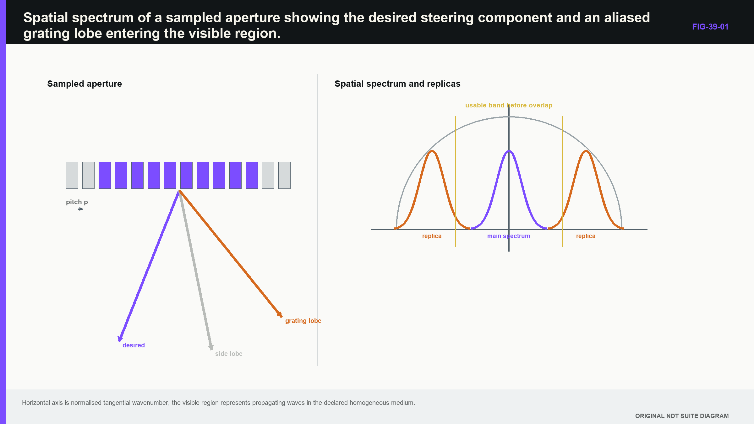
Notice that the unwanted lobe begins with physical aperture sampling before any image processing occurs.
39.2 From element positions to spatial aliasing
A continuous aperture can carry a smooth phase and amplitude distribution. An array represents that distribution at discrete centres. Pitch is therefore a spatial sampling interval, while wavelength sets the phase-change scale in the medium.
Steering shifts the desired spatial frequency away from broadside. Periodic sampling repeats the aperture spectrum at intervals set by reciprocal pitch. When a repeat falls inside the visible region, it represents a direction in which a real wave can propagate. The array can then transmit or receive a strong response from that direction.
Array reviews and manufacturer tutorials identify pitch, wavelength and steering as primary grating-lobe controls. [R014] [R016] Actual level also depends on finite element width, bandwidth, active length, weights, wedge transmission, mode conversion and hardware variation. A pitch equation is therefore a design screen, not final proof of acceptable lobe performance.
The practical sequence is: screen the physical pitch, calculate candidate directions, add realistic element/wedge/bandwidth effects, translate important lobes into component coordinates and then challenge them with complete-system evidence.
39.3 Calculate candidate lobe directions
For an ideal periodic line array, an additional maximum occurs when the phase difference between adjacent elements differs from the intended steering condition by a whole number of cycles. In sine-angle form, the candidate direction is:
| (39.1) Ideal grating-lobe directions for a uniform linear array · EQ-39-01 Where: theta_g = candidate grating-lobe angle from aperture normal; theta_s = intended steering angle; m = non-zero integer lobe order; lambda = wavelength in the represented medium and mode (m); p = element pitch (m) Model limits: infinite periodic linear array; identical point elements; one homogeneous isotropic medium; one harmonic frequency; no wedge or finite-aperture effects |
|---|
Any candidate for which the absolute sine is not greater than one lies in the visible region. Candidates outside that range do not propagate as ordinary plane waves under this model. The equation gives direction, not lobe amplitude.
For a symmetric steering range, excluding first-order ideal lobes gives a convenient pitch screen:
| (39.2) Ideal pitch screen for a symmetric steering range · EQ-39-02 Where: p = element pitch (m); lambda = shortest relevant wavelength in the represented medium and mode (m); theta_max = largest intended steering magnitude from aperture normal Model limits: periodic linear array; homogeneous isotropic medium; point elements; first-order visible grating lobes used as the screening boundary |
|---|
At broadside, this screen becomes p <= lambda. As steering approaches 90 degrees, it approaches lambda/2. Practical designs may need more margin for bandwidth, velocity uncertainty, wedge behaviour and the consequences of a residual lobe.
39.4 Worked design screen across a steering range
| Worked example · Screen pitch for a 60-degree shear-wave range WE-39-01 Given: A linear array has p = 0.60 mm pitch. It is intended to steer shear waves to 60 degrees in steel represented by c = 3,230 m/s at f = 5.0 MHz. Find: Compare the physical pitch with the ideal first-order screen over that steering range. Steps: Calculate wavelength with consistent units. lambda = c/f = 3,230 m/s / 5.0 x 10^6 1/s = 0.646 mm. Calculate the limit: p_max = 0.646 mm / (1 + sin60 degrees) = 0.646/1.866 = 0.346 mm. Answer: The 0.60 mm pitch exceeds the 0.346 mm ideal screen. Technical implication: The simplified model flags significant grating-lobe risk. It does not predict actual transmitted lobe level through the wedge; directivity, bandwidth, refraction and complete-system response still require evaluation. Common mistake: Using the 5 MHz label as the highest relevant frequency or treating a failed screen as acceptable because a display threshold hides the replica. |
|---|
The margin ratio is 0.60/0.346 = 1.73, so this is not a near-boundary rounding issue. A different array, reduced steering range, lower relevant frequency or faster wave mode may change the design. Gain or colour palette cannot correct the spatial ambiguity.
39.5 Element width, kerf and cross-talk
Pitch measures centre-to-centre spacing. Active width plus kerf makes that pitch. Arrays with equal pitch can have different element directivity and active area because their width and gap differ.
Narrower elements radiate over a wider angle but have less active area. Wider elements narrow directivity and may suppress a high-angle grating lobe, while also weakening the desired high-angle beam. The complete first estimate multiplies the ideal array factor by element directivity.
Mechanical or electrical cross-talk can excite response outside the commanded element. The realised aperture then differs from the active-element list. A channel may also have altered phase rather than being simply dead. Element maps and field tests can reveal severe changes, but the target, coupling and processing convention must be controlled.
Elevation remains a second aperture dimension. A linear array can pass its active-axis pitch check while its fixed elevation field misses a skewed target or produces out-of-plane side structure. A matrix array samples in two dimensions; a rectangular or triangular lattice has a two-dimensional pattern of spectral repeats that must be checked across the full steering cone.
39.6 Use the shortest relevant wavelength, not the label
Wavelength decreases as frequency increases, so the highest relevant frequency creates the strictest pitch demand for a fixed mode. A broadband probe contains useful energy above its labelled centre. The assessment should use a measured or justified band and state the amplitude criterion defining that band.
Relevant frequency is shaped by the transducer, wedge, path, attenuation and receive chain. A negligible upper tail may not control, while a strong high-frequency shoulder can. Frequency-resolved plots show that candidate lobe direction moves with wavelength; the time-domain pulse may show a smeared artefact rather than one sharp secondary beam.
Mode matters because shear waves have shorter wavelength than longitudinal waves at the same frequency in common steels. A pitch acceptable for longitudinal steering can fail for shear. Wedge and component both matter: spatial energy generated in the wedge may reflect, transmit or mode convert at the interface. A component-only rule misses this stage.
Anisotropic material changes the visible-region interpretation because phase and group directions are no longer described by one scalar speed. Coarse material can dominate the result through phase distortion and structural noise. Representative-material evidence may then outweigh an elegant isotropic array-factor curve.
39.7 Apodisation trades width, side structure and energy
Uniform weighting uses the full support and commonly gives a narrow main lobe with a characteristic side-lobe pattern. Reducing weights toward the edges lowers some side structure but broadens the main response and reduces coherent gain. That is a physical trade, not a defect in the taper.
Transmit and receive weights combine. Applying a taper on both paths can further reduce side response while widening the two-way point-spread response. The comparison also depends on what is held constant: sum of weights, peak element voltage, total energy or peak main response.
Use at least three metrics: a main-lobe or point-spread width, an unwanted-response measure and a sensitivity or energy constraint. A design that minimises only peak side-lobe level can become broad and weak. A design that minimises only width can produce unacceptable replicas.
Change case: re-normalised taper. A new software version automatically rescales tapered weights to preserve peak image amplitude. Central elements now operate closer to voltage limits, while noise and clipping margin change. The shape name is unchanged, but the physical constraint is not. Regression must compare actual weights, transmitted limits, raw dynamic range and field response.
39.8 Periodic, sparse and aperiodic apertures
Turning off every second element doubles effective periodic spacing and can create strong predictable lobes. An aperiodic sparse pattern spreads unwanted energy into a broader side-lobe floor instead of one dominant repeat. That may be useful, but reduced element count also changes sensitivity, spatial-frequency support and robustness.
Research on compressed sensing shows that reduced sampling can work when the target or data are sparse in a suitable representation and the forward model and regularisation remain valid. [R024] The result depends on sampling pattern and target population; it is not general permission to discard channels.
Structured or plane-wave acquisitions can also exploit redundancy under defined scattering assumptions. Fewer firings may retain useful information, but angular sampling, aperture, signal-to-noise and multiple scattering limit equivalence. [R023] A reduced architecture is a new inspection-system claim requiring validation, not an administrative optimisation.
Sparse optimisation should include position and amplitude tolerances, delay quantisation and credible element failures. Large calibration weights can equalise sensitivity while amplifying noise and reducing dynamic-range reserve. Constrain weight range and keep a practical fault margin.
39.9 Active-aperture clipping and element failure
Requested apertures can be clipped near array ends. A generator may reduce active count, shift the centre or omit laws. Review actual element lists across the sequence. A “32-element aperture” does not exist at a position where the hardware can supply only 20 elements.
Loss of a centre element and loss of an edge element have different consequences. A cluster creates a gap and asymmetric side structure. Robustness studies should use failure patterns found in service, not only random independent failures when connectors or cables create clusters.
Large apertures also span more wedge, surface and material variation. On curvature they may rock or lose contact. In heterogeneous material they may collect larger phase errors. A smaller aperture can be wider in an ideal field yet provide more stable production response.
Failure case: attractive nominal optimum. An optimised 48-element taper gives the lowest simulated side-lobe ratio with perfect channels. One credible three-element cluster raises a replica through the weld-root region above the interpretation-control limit. A 32-element alternative is slightly wider but remains below the limit for the same failure. Robust choice favours the 32-element aperture unless the larger design gains stronger fault detection and release controls.
39.10 Scan-position sampling is a second problem
Element pitch samples the acoustic aperture. Encoder increment samples response as the probe moves. A fine array cannot repair a scan increment that jumps over a narrow target, and fine encoder spacing cannot remove an array grating lobe.
In reconstructed three-dimensional data, the two spatial sampling systems interact. Insufficient scan spacing can repeat or distort along-scan structure. The relevant scale includes target extent, along-scan point-spread response, scanner accuracy and trigger jitter.
Vary scan increment independently during validation. This prevents an encoder artefact from being blamed on the array or a grating-lobe replica from being hidden by interpolation. Stored display pixels are not independent acquisitions.
39.11 Optimise several objectives without hiding the trade
Technique design rarely has one objective. Detection favours energy and angular diversity. Sizing favours stable point-spread behaviour and complementary views. Acquisition speed and data volume favour fewer laws. Robustness favours tolerance to velocity, position and element variation.
A Pareto set contains designs for which improving one declared objective worsens another. Showing the set preserves the trade instead of hiding it inside an unexplained score. Engineering judgement then selects according to the actual priority of coverage, detection, sizing, speed and evidence.
The validation metrics must match the optimisation metrics. If a design was chosen using simulated side-lobe ratio, a trial that records only peak amplitude on one target breaks the evidence chain. Every objective needs a measured counterpart or a clear statement that it remains model-only evidence.
Sensitivity analysis should test whether small plausible change makes another Pareto design clearly better. A selection that flips under minor uncertainty is fragile. Robust optimisation evaluates a distribution or bounded set of realised apertures instead of one perfect nominal curve.
39.12 Turn predicted lobes into component risk
A percentage side-lobe value becomes useful only after its direction and path are mapped into the component. Determine whether the replica meets a back-wall corner, weld root, surface, attachment or target population inside the decision region. The same relative lobe can be harmless outside the component and dominant when it encounters efficient geometry.
Place a strong representative target where its replica crosses a critical region. Record main-to-replica ratio across steering, depth and frequency. Repeat with planned apodisation and failed-element cases. A low free-field lobe can matter when the main path attenuates or the replica forms a corner response.
A controlled diagnostic changes frequency, aperture or steering and predicts how the replica should move. A genuine target should remain at its component coordinate under a valid model. Parameters chosen after seeing the image remain exploratory until the diagnostic rule is validated.
If residual ambiguity cannot be controlled without hiding plausible targets, redesign pitch, frequency, steering range or aperture. A screen threshold cannot restore spatial information sampled ambiguously.
39.13 Evidence boundary and release record
Validation should cover maximum steering, shortest relevant wavelength, aperture transitions, realistic failed-element cases and important elevation or skew boundaries. One depth and centre frequency do not support a broad sector claim. A small target scanned through an arc or field provides angular evidence, but the target-scattering and pulse-echo conventions must be stated.
For a matrix array, inspect the vector tangential wavenumber and the two-dimensional lattice. For a wedge, assess candidate energy before and after the interface. For sparse layouts, repeat with realised positions and sensitivity variation. For encoded scans, test component-motion spacing separately.
The release record states which frequency and steering combination controls pitch margin, where the strongest residual replica lies, how element failure changes it and which validation target exposed the risk. It also records nominal and degraded limits, perturbation assumptions and the region where interpretation controls apply. [R014] [R016] [R023] [R024]
39.14 Evidence-boundary case: a lobe outside one drawing
An active-plane simulation shows the largest replica leaving the two-dimensional weld section without touching the inspection region. On that drawing it appears harmless. The physical target, however, is finite in length and the probe has a fixed elevation aperture. A three-dimensional calculation places part of the replica on a nozzle transition outside the modelled slice, where it can return a strong geometric response.
The original conclusion failed because “outside the component” really meant outside one selected plane. The appropriate evidence extension is not simply another active-plane map. It includes the elevation field, component surface model, skewed target positions and registration tolerance. A measured target or geometry feature should challenge the predicted three-dimensional path.
This case also shows why an interpretation rule cannot be separated from field evidence. If the replica moves predictably when aperture or frequency changes, a controlled comparison may distinguish it from a physical target. That rule is useful only inside the tested geometry and signal-to-noise range. Outside the demonstrated region, the correct action is escalation or redesign, not confident rejection of the response.
The evidence boundary should be visible in the technique: steering and aperture ranges, component region, relevant frequency band, allowed channel condition and the diagnostic rule. A lobe analysis that cannot be connected to those controlled quantities remains developmental engineering, however polished its spectrum plot appears.
39.15 Practical release check across the complete law set
Before release, sort the law set by the variables that drive spatial aliasing: steering magnitude, relevant upper frequency, active aperture and realised channel pattern. Review the combinations nearest the predicted boundary rather than checking only the centre law. Confirm that any diagnostic response used by operators remains visible with expected noise, coupling and display settings.
Repeat the screen after a credible failed-element pattern and at aperture transitions. If the strongest residual lobe moves into a geometry feature or target region, document the resulting restriction or redesign. This final check connects the mathematical screen to the actual law file and prevents a safe nominal array calculation from being applied to a different realised aperture.
39.16 Substitution case: equal pitch does not mean equal sampling behaviour
Two linear probes have the same nominal pitch and element count. The proposed replacement has wider elements, narrower kerfs and a different measured centre-frequency band. Applying the same pitch equation produces the same geometric candidate lobe directions, yet the measured lobe levels and main-response widths differ.
The pitch equation locates ideal replicas under its assumptions. It does not predict how strongly finite elements radiate into those directions. Wider elements change element directivity. The shifted frequency band changes wavelength and the part of the pulse that approaches the sampling boundary. Construction and matching layers can also change sensitivity across steering.
Compare the probes with one declared aperture and normalisation. Review measured spectrum, element response, field width and replica level across the released steering range. Include the upper effective frequency that carries useful target response, not merely the frequency printed on the case.
Now introduce a credible channel fault. A failed edge element changes effective taper and main-response symmetry. A failed internal element creates a different aperture discontinuity. The replacement may be more sensitive to one pattern even when both probes pass a simple element-amplitude tolerance.
Finally place the residual field in component coordinates. If the stronger replica intersects a root, counterbore or nozzle transition, challenge that feature during validation. If it remains outside the qualified volume only under ideal placement, add registration tolerance before accepting the conclusion.
Substitution is therefore output specific. Main-beam location can remain comparable while false-call behaviour, boundary sensitivity or resolution changes. Equal pitch supports the first sampling screen; realised aperture and component evidence support the release. [R014] [R016] [R023] [R024]
The release record should state the comparison uncertainty and normalisation. A 2 dB lobe difference is not meaningful when remounting varies by the same amount. Repeated maps and reference scans separate stable construction differences from coupling scatter, while preserving any region where the result remains too variable for a substitution claim.
In plain words
- Element pitch samples phase across the aperture, and excessive spacing can create a real unwanted beam.
- Correct focal delays do not guarantee that the aperture is sampled without spatial ambiguity.
- The shortest relevant wavelength and largest steering magnitude normally create the strictest pitch case.
- Element width, kerf, bandwidth, wedge transmission and wave mode change actual lobe level.
- Apodisation trades main-response width, side structure and energy.
- Sparse and aperiodic apertures redistribute information and need their own validation.
- The realised active elements and credible failures matter more than a nominal aperture label.
- Residual lobe risk is judged in component coordinates against real geometry and target populations.
Formal synthesis
Spatial-sampling theory connects periodic element positions with repeated aperture spectra. Ideal lobe-direction and pitch equations provide conservative screens under homogeneous point-element assumptions. Level 3 design then adds finite elements, broadband response, wedge and mode transmission, sparse selection, realised-channel variation and scan-position sampling. Aperture optimisation is multi-objective, and release evidence must show that residual aliases remain controlled in the intended component rather than merely low on an ideal plot.
Key terms
- Spatial sampling: discrete representation of the aperture at element positions.
- Visible region: directions that support propagating waves in the stated model.
- Grating lobe: strong repeated beam created by periodic spatial aliasing.
- Sparse aperture: deliberate subset of available element locations.
- Aperiodic aperture: non-repeating selection used to redistribute replicas.
- Pareto set: designs with explicit unresolved trade-offs among objectives.
- Robust optimisation: selection tested against credible realised variation.
Key relationships
- EQ-39-01 predicts ideal candidate lobe directions, but not their actual amplitude.
- EQ-39-02 screens pitch using the shortest relevant wavelength and maximum steering magnitude.
- Wavelength decreases with frequency, so broadband upper content can control pitch risk.
- Array pitch and encoder increment are separate spatial-sampling intervals.
Common mix-ups
- Side lobes from finite aperture are not identical to periodic grating lobes.
- Element width is not element pitch; kerf separates them.
- More active elements do not correct excessive physical pitch.
- Lower displayed replica amplitude is not proof that ambiguity has been removed.
- Fine image pixels are not fine acoustic or encoder sampling.
Bridge to Chapter 40
Chapters 37–39 have controlled the field, law timing and spatial aperture. Chapter 40 adds motion and time: the instrument must complete every law and group at the correct encoder position while buffers, clocks and storage remain healthy. A perfect aperture is little comfort if the scanner quietly skips complete frames.
Sources and further study
- [R014]
- [R016]
- [R023]
- [R024]
Study and revision only. This is not an approved inspection procedure, acceptance criterion or qualification.