
CHAPTER 55 · FMC / TFM / PCI Level 3
Matrix-Acquisition Architectures
In this chapter · 28 sections
Why this matters
A Level 2 learner already knows the full matrix as a grid of transmit-receive A-scans. Level 3 must decide whether every cell still needs to be measured. Fewer firings can shorten a scan and reduce storage, but a missing trace is not something reconstruction can simply invent. The first task is therefore to see exactly what each acquisition records, what it infers and what it loses.
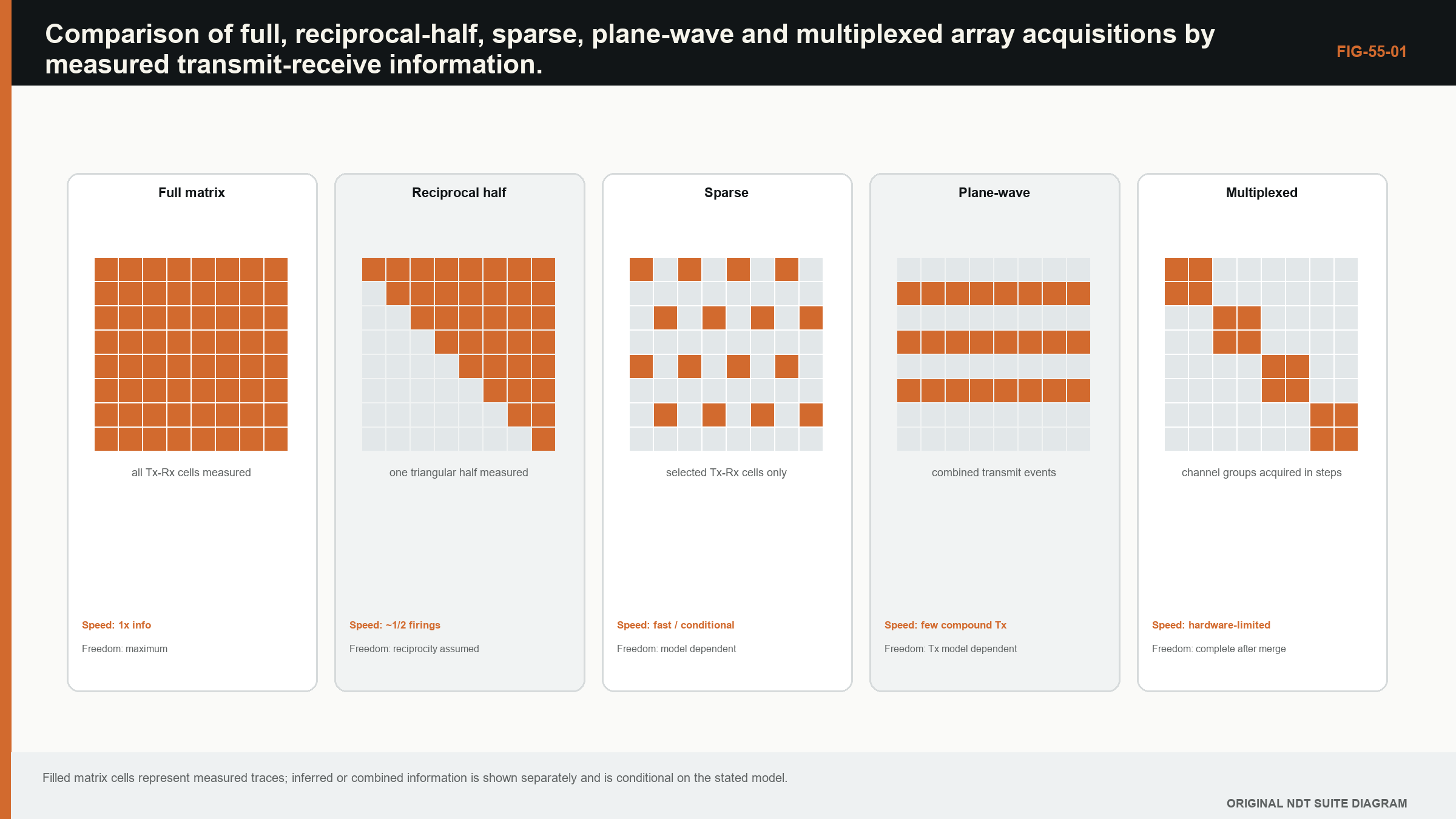
Picture a four-element probe. A full acquisition records sixteen ordered cells. A reciprocal-half acquisition records one triangular half and treats the opposite half as equivalent after validation. A sparse acquisition records selected cells. A plane-wave acquisition sends a broad field from several elements together, so it is a different measurement basis rather than a partly empty full matrix. This picture comes before rank, identifiability or inverse-problem language.
What you already need
- An FMC cell contains one A-scan for one transmitter and one receiver.
- TFM selects a predicted time from many cells to calculate an image point.
- Phase, gain, range, coupling and position can be damaged during acquisition.
- A reconstruction can be repeated only with information that was actually retained.
What you will learn
You will compare full, half, sparse, synthetic-aperture and plane-wave acquisition; calculate basic pair counts; explain which assumptions make a reduction defensible; recognise permanent information loss; and design a challenge test that can expose a weak architecture.
Words you will meet
Acquisition architecture means the planned pattern of transmissions, receivers, samples and positions that creates the dataset. Reciprocity is the physical expectation that a path behaves the same when transmitter and receiver are exchanged under stated conditions. Sparse means deliberately retaining only part of the possible measurement grid. Identifiability means whether different physical situations remain distinguishable in the retained data. Optionality is the ability to apply another valid reconstruction or diagnostic later because the necessary raw information was kept.
The Level 3 step
At Level 2 the learner checks whether a dataset is usable. At Level 3 the learner justifies why a proposed dataset contains enough information for the intended targets and decisions. Formal measures appear later in the chapter, but each one must still answer a plain question: which distinction in the component can the acquisition preserve, and which distinction has it made impossible to observe.
55.1 Acquisition architecture defines the available inverse problem
An array acquisition is a set of transmitted fields, received channels, time samples and positions. The architecture determines which parts of the array response are observed before any image is formed. Reconstruction can reorganise and combine recorded information; it cannot recover distinctions that the acquisition never encoded unless additional assumptions make those distinctions inferable.
Full matrix capture fires each selected transmitter and records every selected receiver. For N elements with all used in both roles, the ordered matrix contains N^2 traces per position. This data supports flexible post-processing because transmit and receive pairs remain explicit. The original TFM formulation uses that flexibility to focus synthetically at each image point. [R017]
Calling an acquisition full does not guarantee quality. Time range, sampling, gain, phase, channel health, element position and metadata still control usable information. Conversely, a reduced architecture is not automatically inferior. It can be efficient when its assumptions match the scattering problem and its retained measurements support the intended outputs.
55.2 Full and half matrices
In a linear reciprocal medium with interchangeable transmit and receive behaviour, the impulse response from element i to j is expected to equal the response from j to i after appropriate channel corrections. The matrix is then symmetric in principle. Recording one triangular half plus the diagonal can reduce firings or storage if the acquisition hardware and intended processing can use that symmetry.
Reciprocity is a physical relationship, not a guarantee that measured traces are identical. Transmit and receive electronics can differ by channel. Multiplexing paths, pulser output, receiver gain, saturation and noise can break measured symmetry. Motion between reciprocal acquisitions also changes the component state seen by the array. A reciprocity residual is therefore both an assumption check and a diagnostic.
| (55.1) Reciprocal half-matrix trace count including diagonal · EQ-55-01 Where: N_half = unique unordered transmit-receive pairs including self-pairs; N = number of elements used in both roles Model limits: pair order can be inferred through validated reciprocity and diagonal traces are retained |
|---|
If only storage is reduced after a complete acquisition, speed may not improve. If firings are reduced, SNR and channel diagnostics can change. The technical record should distinguish acquisition reduction from lossless file packing or symmetry-aware reconstruction.
55.3 Sparse and reduced matrices
A sparse matrix retains selected transmit-receive pairs. Selection can be random, structured, aperture-based, distance-based or optimised for a target region. Removing far-offset pairs reduces aperture diversity. Removing diagonal pairs can reduce strong near-surface or common-mode information but also removes useful diagnostics. The matrix pattern shapes the point-spread response and sensitivity to target orientation.
Structured periodic subsampling risks coherent aliases. Aperiodic patterns can spread artefact energy, but reconstruction then relies on the irregular sampling model. Compressed-sensing approaches exploit sparsity in a chosen domain and can reduce data when the forward model and regularisation match the problem. Performance depends on sampling pattern, SNR and how sparse the scene truly is. [R024]
Reduction should be evaluated against outputs, not visual resemblance. Detection, localisation, sizing, artefact rejection and uncertainty may respond differently. A sparse acquisition that preserves one isolated point target can fail for extended planar reflectors or multiple scattering.
55.4 Synthetic-aperture acquisition
Synthetic-aperture focusing techniques acquire data from sequential spatial positions or subapertures and combine them as a larger effective aperture. The aperture can be formed by moving a single element, stepping a small group or using array elements. The method trades acquisition sequence and motion control for post-processing flexibility.
Position accuracy becomes part of phase coherence. An error small compared with image scale can be large compared with wavelength. Motion during a transmit-receive event can also matter in high-speed systems. The synthetic aperture is only as accurate as the element-position and timing record used in reconstruction.
Sparse synthetic apertures can reduce hardware channels, but they may require longer scan time or stable coupling across more positions. A design should include motion repeatability, coupling variation and the target's stationarity, not only nominal aperture length.
55.5 Plane-wave acquisition
Plane-wave imaging transmits a broad steered wave using many elements together and records receive channels. Repeating several transmit angles provides angular diversity. Receive focusing is then applied in reconstruction. Because one plane-wave firing illuminates a broad region, far fewer transmissions may be required than element-by-element FMC.
Research on multimodal plane-wave imaging shows that steered plane waves can support multiple propagation modes and views, but reported reductions are specific to the tested arrangements. [R022] Studies of acquisition strategy show that under single-scattering assumptions, FMC contains structured redundancy and plane-wave sets can retain useful information with fewer firings. Angular sampling, aperture, SNR and target scattering govern the equivalence. [R023]
Plane waves distribute transmit energy differently from single-element firings. Peak voltage, total aperture energy, safety limits, near-surface response and saturation may change. Comparing images at equal display gain does not ensure equal acoustic or electronic conditions.
55.6 Multiplexing and channel limits
Many instruments have fewer parallel channels than probe elements. Multiplexers connect subsets to pulsers and receivers. Switching time, path impedance, protection recovery and channel mapping can influence timing and amplitude. A nominal 128-element probe on a 32-channel instrument may require several subcycles to populate one acquisition.
The schedule determines frame rate and susceptibility to motion. If reciprocal or related traces are recorded at widely separated times, coupling or position can change between them. Channel reuse can also make a hardware fault appear in a patterned set of matrix cells. A matrix health plot indexed by physical element and electronic channel can separate these causes.
Multiplexing identity belongs in metadata. Element number, connector pin, pulser path and receiver path may not be one-to-one. A file that stores only a trace index cannot support later diagnostics reliably.
55.7 Compression assumptions
Compression may be lossless, near-lossless or model-based. Lossless compression changes representation but preserves exact samples. Near-lossless schemes quantise or transform data within a tolerance. Model-based compression retains features or coefficients believed sufficient for a reconstruction.
The acceptable method depends on future use. If raw phase supports coherence imaging, compression must preserve phase within a validated bound. If data may be reprocessed with new paths, storing only one image is not equivalent to storing matrix traces. A small file is not evidence of efficient acquisition if it discards the audit trail.
Compression performance should be measured on representative noise, targets and artefacts. Smooth synthetic signals often compress better than grain-noise data. Error metrics should include waveform, phase, image and decision effects rather than byte ratio alone.
55.8 Identifiability and information loss
Identifiability asks whether different physical states can produce indistinguishable retained data. If two target configurations map to the same reduced measurements, no reconstruction can separate them without prior assumptions. A colourful algorithm can choose one solution, but the acquisition did not identify it.
Rank and singular-value analyses of a linearised forward model can reveal poorly observed combinations. Fisher-information or sensitivity measures can guide acquisition design when noise models are available. These tools depend on the target and model. A design optimised for point scatterers may not identify extended cracks.
Information loss can also be diagnostic. Omitting self-pairs may remove sensitivity to near-surface coupling. Omitting long offsets may reduce angular diversity. Recording only envelopes removes RF phase and polarity. The architecture should list what is intentionally unavailable.
55.9 Designing and validating an architecture
Begin with target population, component, required views, outputs and constraints. Select candidate transmissions and receivers. Predict coverage and point-spread behaviour. Test robustness to noise, velocity, geometry, channel loss and multiple targets. Compare with a fuller reference acquisition where practical.
Validation should include cases designed to expose the reduction assumption. For reciprocity, introduce known channel asymmetry. For sparse sampling, test extended and multiple targets. For plane waves, test angular extremes and saturation. For compression, test phase-sensitive reconstruction and raw-data diagnostics.
The source file should retain architecture version, element maps, transmission definitions, sample settings, trigger sequence and any inferred symmetry. Self-describing containers such as HDF5 can store multidimensional arrays and attributes, but the NDE semantics still have to be designed and governed. [R053]
| Worked example · Trace reduction from a reciprocal half matrix WE-55-01 Known: An array uses 128 elements as both transmitters and receivers. Compare the ordered full matrix with a reciprocal triangular half including diagonal pairs. Find: Trace counts and percentage reduction. Method: Full count is 128^2 = 16,384. Half count is 128(129)/2 = 8,256. Reduction is (16,384 - 8,256)/16,384 = 49.6%. Result: The reciprocal half contains 8,256 unique unordered pairs, about 50.4% of the full ordered matrix. Engineering meaning: The arithmetic does not prove equivalent measured data. Channel asymmetry, motion and non-reciprocal implementation effects must be bounded before omitted pairs are inferred. |
|---|
Guided Level 3 case: reducing a weld acquisition
A proposed weld technique uses a 64-element linear array. The reference dataset is a complete FMC acquisition. Production speed is too slow, so three alternatives are considered: a reciprocal half matrix, every second transmitter with all receivers, and a small set of plane waves. The Level 3 task is not to select the smallest file. It is to decide what must remain observable for the intended weld targets and for later diagnosis.
First list the required outputs. The technique must detect and position planar sidewall and root targets, retain enough path diversity to distinguish known geometry, and preserve RF data for a phase-sensitive complementary image. It must also reveal weak or dead elements. These requirements immediately rule out storing only a finished envelope image, because that choice removes phase and cell-level diagnostic evidence.
Next compare what each candidate measures. The reciprocal half retains every unordered element pair but infers the reversed order. It therefore needs evidence that transmit and receive paths are sufficiently interchangeable after channel correction. The every-second-transmitter design retains all receivers but changes transmit aperture sampling and target illumination. The plane-wave set uses broad transmissions and angular sampling, so it must be compared as its own acquisition rather than treated as missing FMC cells.
Use the full dataset for retrospective screening. Reconstruct every required view with fixed display and measurement rules. Compare target coordinate, response spread, artefact location and phase-derived output. Remove an additional channel deliberately and repeat the test. This shows whether the design degrades gradually or fails suddenly. Retrospective results are only the first gate because they do not reproduce native transmit energy, switching schedule or motion.
The second gate is native acquisition on representative specimens. Repeat scans at operating speed and include difficult target orientations, geometry responses and realistic coupling change. Record firing definitions, element maps, pair-validity masks and timing. If a candidate passes easy side-drilled holes but loses the planar target or hides a bad channel, the reduction is not supported for the stated technique.
The conclusion names the selected architecture and its boundary. It identifies inferred reciprocal data, absent transmissions, preserved RF phase, validated target population and stop rule after further channel loss. This is a defensible reduction because it explains retained and lost evidence instead of presenting speed as proof of equivalence.
55.90 Technical extension: architecture comparison on common information units
55.90.1 Transmission bases
Element firings and plane waves can be viewed as different transmission bases. If the transmitted fields span the same relevant subspace and measurements are linear with adequate SNR, one dataset may be transformed toward another. Finite aperture, hardware limits and scattering complicate this ideal. The condition number of the transformation indicates noise amplification.
This view explains why the number of firings alone is not information count. Closely spaced plane-wave angles can be redundant, while a small set chosen across the aperture spectrum can be informative. Element firings provide localised basis functions but may have lower transmit energy.
55.90.2 Reciprocity audits
Before relying on a half matrix, measure reciprocal residuals over time, amplitude and phase. Summaries should retain distributions and channel patterns, not only a global average. A small mean can hide one bad channel that affects a critical view.
Residual tolerance should be derived from impact on reconstruction and target metrics. If phase-coherence imaging is intended, a phase residual can matter even when amplitude images look similar.
55.90.3 Missing-data maps
Reduced and faulted acquisitions should carry an explicit pair-validity mask. Zero-filled missing traces are not true zero measurements. Reconstruction can use pair-count normalisation and uncertainty or artefact estimates based on the mask.
Architecture validation should include the actual mask after multiplexing and rejected channels. A design optimised for an ideal sparse pattern may degrade when an additional element fails.
55.90.4 Future-use boundary
An acquisition optimised for one reconstruction may prevent later methods. Envelope-only storage blocks RF phase analysis. A narrow time gate blocks deeper paths. A reduced transmit basis can limit a newly identified target orientation.
The retention decision should state expected future uses and accepted irreversibility. Where long-term evidence is important, a richer raw acquisition can be justified even if routine images use a reduced subset. [R017] [R022] [R023] [R024] [R047] [R053]
55.91 Quantifying architecture equivalence
Architecture equivalence should be tested at several layers. At data level, compare whether the reduced measurements can predict omitted full-matrix traces within a bounded residual. At image level, compare coordinate, PSF, amplitude and artefacts under fixed reconstruction. At decision level, compare detection, sizing and false calls over the intended population.
The tests are nested but not interchangeable. A small waveform residual can matter to PCI phase. Similar images can produce different measurements at a threshold. Similar decisions on easy targets can hide lost sensitivity near the boundary.
Use a full acquisition as a reference where feasible and derive candidate reductions from it. This controls component and coupling while comparing pair sets. A second experiment should acquire the reduced scheme natively to include transmission energy, timing and motion differences that retrospective subsampling omits.
For plane-wave equivalence, examine the conditioning of the transform between element and plane-wave bases over the usable aperture. Noise amplification and finite angular range can make theoretical inversion unstable. Report which target spatial frequencies or angles are weakly observed.
An architecture release should include a missing-pair policy. If additional channels fail, state whether reconstruction stops, degrades with a warning or switches to a separately validated pattern. Silent continuation changes the effective architecture without review. [R017] [R022] [R023] [R024]
55.92 Architecture uncertainty and retained optionality
Represent architecture uncertainty through pair-support and transmission-basis perturbations. Remove plausible additional channels, add timing and gain variation, and test target and artefact populations. Report which outputs degrade first. This identifies whether the design has graceful degradation or a cliff.
Optionality has value when raw data may support future paths or algorithms. Quantify its storage and acquisition cost rather than treating it as free. A project can retain full data on selected qualification and high-consequence cases while using reduced acquisitions elsewhere, provided the boundary and rationale are controlled.
Data containers should store physical element and transmission definitions, not only matrix dimensions. Plane waves, sparse apertures and multiplexed groups need explicit basis metadata. Without it, a future processor cannot distinguish unmeasured information from zero response.
Architecture review should include an information-loss statement in plain language: which reciprocal directions are inferred, which offsets are absent, whether RF phase is preserved, which time range is unavailable and which views cannot be formed. [R017] [R022] [R023] [R024] [R053]
55.93 Architecture release question
Before accepting a reduced architecture, identify a target or fault case for which the omitted information would matter and demonstrate the planned control. If no such challenge can be articulated, the reduction assumptions are not yet understood well enough for a broad capability claim. [R023] [R024]
55.94 Native-acquisition confirmation
After retrospective reduction demonstrates feasibility, acquire the architecture natively at operating speed. Compare timing, transmit energy, motion sensitivity and channel mapping with the full reference. This closes the gap between deleting data after collection and never measuring it. [R022] [R023]
Chapter synthesis
Matrix architecture determines what information exists before reconstruction. FMC preserves ordered transmit-receive traces; reciprocal half matrices reduce data only under validated symmetry. Sparse, synthetic-aperture and plane-wave methods trade acquisition burden against assumptions and spatial information. Multiplexing couples timing and channel identity to motion. Compression must be judged against phase, future processing and provenance needs. Identifiability analysis and adversarial validation reveal what a reduced architecture cannot distinguish. Efficiency is defensible only when the intended detection, location, sizing and diagnostic outputs remain supported.
Key equations and relationships
| (55.2) Reciprocity residual for a trace pair · EQ-55-02 Where: e_ij = residual; x_ij and x_ji = reciprocal measured traces; g_ij = declared amplitude correction; Delta_t_ij = declared timing correction Model limits: common component state and position, corrections established independently and a reciprocal linear propagation regime |
|---|
In plain words
- The chapter's central control is architecture, and its meaning must be stated before its mathematics or software implementation.
- A faster, sharper or cleaner result is not automatically a more reliable result.
- Every claimed improvement depends on a declared dataset, model, configuration and target population.
- Known reference cases and deliberately difficult cases reveal different weaknesses.
- Stored raw evidence, metadata and software identity make later review possible.
- The technical conclusion must remain inside the boundary demonstrated by the evidence.
Key terms in this chapter
The words introduced at the chapter opening are the minimum vocabulary for its Level 3 work. Use them consistently in the technique, validation record and report. Where a supplier uses a different label, record the supplier term without allowing it to replace the physical definition.
Common mix-ups
- Do not confuse a similar displayed image with equivalent retained information.
- Do not confuse software verification with physical validation of an inspection technique.
- Do not confuse an assumed model output with a directly observed quantity.
- Do not confuse a demonstrated result for one target population with universal capability.
Independent review checkpoint
Give a second competent reviewer the raw or reference data, the declared architecture method, the controlled configuration and the expected comparison outputs. The reviewer should be able to reproduce the important result without using an undocumented display adjustment or private software setting. Record the version, input identity, contributor or channel mask, model inputs, numerical tolerances and any excluded cases. Also record one observation that would contradict the preferred explanation. Where the result supports a decision, the reviewer records the nearest failure boundary and one realistic change that would trigger revalidation. This checkpoint does not turn independent review into a ceremonial signature. It tests whether the evidence chain is understandable, repeatable and honest about its limits.
Bridge forward
Chapter 56 turns the retained measurements into image values and shows why the exact calculation must be declared.
Sources and further study
- [R017]
- [R022]
- [R023]
- [R024]
- [R047]
- [R053]
Study and revision only. This is not an approved inspection procedure, acceptance criterion or qualification.