
CHAPTER 5 · FMC / TFM / PCI Level 2
FMC Acquisition and Data Integrity
In this chapter · 17 sections
Learning outcomes
After completing this chapter, the learner should be able to:
describe a complete conventional FMC firing and receiving sequence;
distinguish full, half-matrix, sparse and other reduced acquisition strategies;
select a defensible time range, sampling rate, bandwidth and digitisation range;
verify element activity, coupling, matrix completeness and encoder integrity;
estimate raw data volume and recognise file-overhead limits;
explain acquisition-speed, data-quality and storage trade-offs;
define minimum metadata needed for later reconstruction; and
decide when data must be reacquired rather than reprocessed.
Crossover map
| Encoded PAUT control | FMC acquisition extension | Main integrity risk |
|---|---|---|
| Focal-law sequence | Transmit-receive matrix sequence | Missing, repeated or misassigned pair traces |
| PRF and scan speed | Complete matrix cycle per position | Moving before the matrix is complete |
| Gate/time range | Pair waveform record length | Relevant long or skip paths omitted |
| Receiver gain and filter | Applied across many elementary traces | Strong pairs clip while weak pairs remain near noise |
| Element check | Row/column matrix-health check | Subtle pair-dependent loss is hidden in the final image |
| Encoder increment | Position-linked matrix data | Large files contain duplicated or skipped positions |
| Setup and data file | Raw matrix, metadata and reconstruction versions | Result cannot be reproduced after software changes |
What an FMC acquisition actually records
At one physical scan position, a conventional pulse-echo FMC sequence proceeds in steps:
connect or select the first transmitting element;
fire the pulse;
record the selected receive elements over the defined time range;
store those A-scans with transmitter and receiver identities;
select the next transmitting element; and
repeat until the required matrix is complete.
Link the complete cycle to an encoded position and repeat it along the scan. The record therefore has transmitter, receiver, time and position dimensions plus essential metadata.
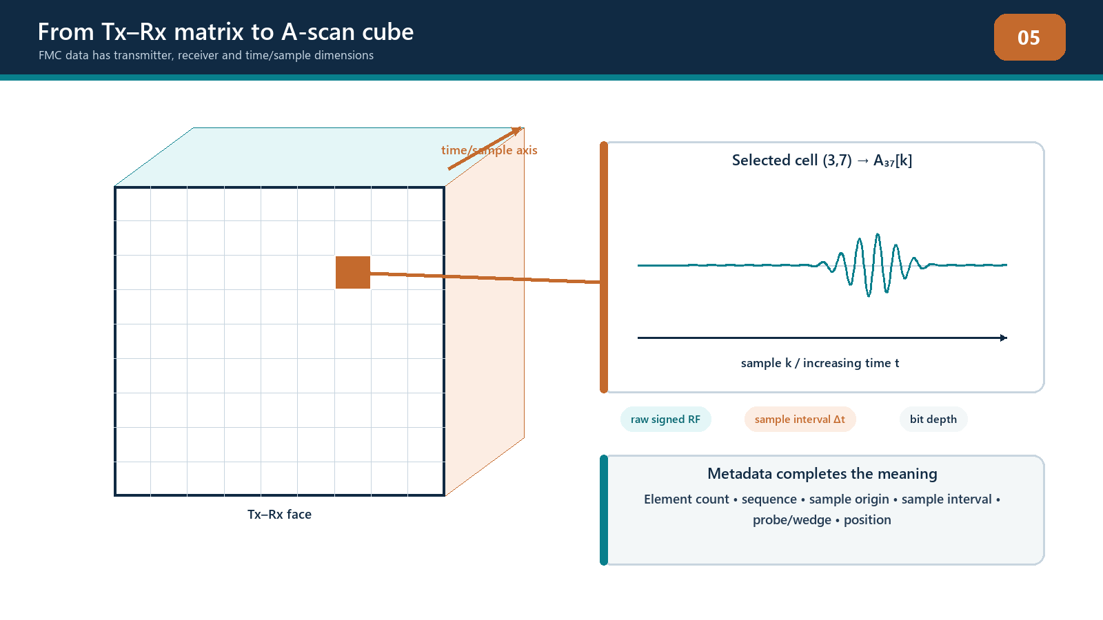
Hardware may use parallel receivers, multiplexing or other arrangements. The technician need not design the electronics, but must know what was recorded. A TFM-labelled screen can originate from full FMC, half-matrix, sparse, plane-wave or another documented acquisition. Identify the actual acquisition in the technique and report.
Full, half and reduced matrices
Full matrix
A full matrix records every defined ordered pair: commonly, each selected element transmits and receives. It provides pairwise flexibility but demands time, storage and processing.
Half matrix
A half matrix records one diagonal half of a nominal reciprocal matrix and handles self-pairs explicitly. It relies on demonstrated reciprocal conditions and is not automatically equivalent to full FMC.
Sparse or reduced matrix
Sparse acquisition records selected transmitters, receivers or pairs to increase speed or reduce data. The selection may be regular, optimised or proprietary. Its performance can be excellent for a defined task, but it changes effective aperture, spatial sampling, lobe behaviour and traceability. Name the reduction and demonstrate the intended detection, location, resolution and sizing performance.
Other acquisition families
Plane-wave imaging and other advanced schemes transmit with multi-element laws and reconstruct from the received elementary data. They can support TFM-like or PCI processing on some systems, but they are not conventional one-element-at-a-time FMC. The course uses FMC as the primary foundation and treats other families as separately controlled methods.
The acquisition signal chain
Pulser
Pulse voltage, pulse width, damping and repetition control affect transmitted energy and frequency content. Excess energy can saturate the receiver or produce long ring-down; insufficient energy can leave long paths below the usable noise margin. Settings should match the array and approved technique.
Array and coupling path
The pulsed element sends energy through its probe backing, matching layer, wedge or couplant and into the component. Every interface can affect bandwidth, delay and amplitude. Uneven wedge contact can change contributions across the aperture. Surface roughness can vary coupling as the array moves.
Receiver and analogue filtering
Receive gain places the electrical waveform within the digitiser's usable range. Analogue filtering limits unwanted frequency content before sampling. If gain is too high, strong traces clip. If it is too low, weak traces fall near noise. One gain setting may have to accommodate very different diagonal and wide-pair responses.
Digitiser and storage
The digitiser samples the waveform at defined intervals and bit depth. Digital filters, averaging, compression or rectification may occur before storage. These operations can change amplitude, phase and later processing options. The retained data representation must be known.
Selecting time range and sampling
Acquisition time range must cover the longest relevant transmit-plus-receive path, including wedge legs, skips, converted modes and verification targets. Add suitable allowance for tolerances and model variation without collecting unlimited irrelevant reverberation. A range selected for direct PAUT beams may be too short for wide off-diagonal or skip-path pairs.
The sampling rate should represent the retained signal bandwidth with adequate timing fidelity. Higher sampling creates more samples and larger files. It does not increase the probe's acoustic bandwidth. Reduced sampling can save storage but can distort timing and phase if it is insufficient for the processed frequency content.
Record the acquisition origin. Electronic delay, pre-trigger, wedge time and material time are not interchangeable. A reconstruction must know how stored sample index maps to physical travel time.
Gain, clipping and usable phase
Amplitude-free PCI does not use conventional echo amplitude as its image value, but its phase estimate still comes from acquired waveforms. Three acquisition zones matter:
below useful signal-to-noise: phase is dominated by noise and unstable estimates;
within the digitiser range: waveform form, timing and phase are retained; and
clipped or saturated: the original waveform shape has been lost.
No display algorithm can prove that data remained within range unless underlying channel checks or acquisition diagnostics support it. Check representative strong diagonal/near-surface pairs and weak long-path pairs. If one group clips before another becomes usable, probe, pulser, receiver, aperture or acquisition choices may need reconsideration.
Digital normalisation can make traces or images appear equally strong. It does not repair low signal-to-noise ratio, clipping or missing bandwidth. Always distinguish display convenience from measurement integrity.
Channel and matrix checks
Before scanning, verify:
probe identity, frequency, element count and element map;
wedge identity, orientation and coupling face;
transmitter and receiver selections;
row and column activity on a stable reference target;
channel timing consistency;
absence of unacceptable cross-talk or saturation;
matrix dimensions and sequence completeness; and
stability over repeated acquisitions.
An element check designed for PAUT may remain useful, but FMC adds pair-pattern evidence. A weak element can affect a row and column, while electronic problems may affect only transmit or receive behaviour. Retain the check output where the quality system requires it.
Pair exclusions should not be used casually to make an image cleaner. Record which pairs were excluded, why, how the change affects aperture and whether the resulting technique remains within its demonstrated range.
Coupling and surface control
FMC acquisition is sequential, so conditions should remain stable while the matrix is recorded. If the probe moves significantly or coupling changes during one cycle, the matrix no longer represents one acoustic state at one position. This can reduce reciprocity, blur reconstruction and create coherence artefacts.
Check:
contact over the full wedge or probe face;
couplant film stability;
surface scale, weld spatter, profile and curvature;
probe rocking or lift-off;
temperature effect on wedge, couplant and component velocity; and
mechanical stability during stationary and encoded acquisition.
When scanning by hand, excessive speed can allow the probe to travel appreciably during a matrix cycle. Encoded systems can also trigger positions faster than complete matrices can be acquired. The approved technique should set a maximum speed or acquisition condition tied to matrix completion and position increment.
Encoder and position integrity
The encoder links each matrix to component coordinates. Verify distance calibration, direction sign, index offset and scan origin before acquisition. During scanning, monitor for wheel slip, lift, backlash, missed triggers, repeated positions and motion reversal.
Position increment should support the required scan-direction sampling. A small reconstruction pixel does not compensate for a coarse physical scan increment. Conversely, an unnecessarily tiny increment increases file size and scan time without guaranteed acoustic benefit.
Use physical coverage marks or independent measurements where practical. The final dataset should show expected start, end and overlap positions. A complete matrix attached to the wrong coordinate is still invalid evidence.
Data-volume estimation
For a simple uncompressed estimate, define the number of encoded positions, transmitters, receivers, samples per trace and stored bits per sample. The nominal raw payload is:
B_frame = N_pair N_s b / 8; B_dataset = N_pos N_pair N_s b / 8 bytes
For example, 1,000 positions, 64 transmitters, 64 receivers, 2,000 samples and 16 bits per sample produce approximately 131 billion bits, or about 16.4 GB, before headers, indexes, checksums and other overhead. File compression or reduced acquisition can lower storage, while multiple groups and metadata can increase it.
Estimate this before field work. Confirm storage, transfer time, processing limits, review capacity, backup and retention. Filling the instrument before completing the scan is innovative only in the submarine-with-screen-doors sense.
Metadata and configuration control
To reproduce acquisition, preserve:
component and examination identifiers;
probe, wedge, cable and instrument identities;
software/firmware version;
element map and matrix scheme;
pulser and receiver settings;
sampling, filtering, averaging and stored signal type;
time range and origin;
coordinate origin, encoder scale, direction and increment;
material velocities, thickness and surface model;
operator, date, temperature and coupling notes;
setup revision and approval status; and
pre-use and post-use check results.
Use checksums or the quality system's integrity control when transferring large files. Preserve the original acquisition separately from derived reconstructions. If data are converted for another software package, record the conversion tool, version and any information that is lost.
Reacquire or reprocess?
Reprocessing can correct or investigate:
an approved change to velocity or geometry model;
a different justified path or region;
display range, colour or annotation;
a validated pair weighting or exclusion; and
alternate amplitude or coherence processing supported by retained data.
Reprocessing cannot validly recover:
time ranges that were not recorded;
channels that never fired or received;
waveform shape destroyed by clipping;
position information lost through encoder failure;
missing scan coverage;
unstable coupling during acquisition; or
frequency content removed before storage.
When the missing evidence is an acquisition problem, reacquire while conditions and component access allow. A later image-processing rescue attempt is rarely improved by the passage of time.
Field workflow: controlled FMC acquisition
Before scanning
Confirm the approved technique, component identity and examination extent.
Verify probe, wedge, element map, instrument and software revision.
Load the controlled acquisition and reconstruction configuration.
Confirm matrix type, dimensions, time range, sampling and stored signal form.
Complete channel, timing, saturation and reference-target checks.
Calibrate encoder distance, direction and origin.
Estimate file size and confirm storage/backup capacity.
During scanning
Maintain coupling and full contact.
Remain below the demonstrated scan speed.
Monitor position, matrix rate, dropped-data indicators and raw-signal range.
Confirm coverage, overlaps and physical obstructions.
Pause and investigate any discontinuity that follows scan motion or coupling rather than component geometry.
After scanning
Confirm expected position count and spatial extent.
Review matrix health and selected RF traces.
Repeat required reference and channel checks.
Save the original data under a unique controlled identifier.
Verify transfer integrity and record the reconstruction recipe separately.
Document any limitation, rescan or technical disposition.
Practical 5 - Acquire and disposition an FMC dataset
Objective
Plan, acquire and audit an encoded FMC dataset that is fit for a defined teaching reconstruction.
Resources
documented instrument, array and wedge;
reference target and representative scanned specimen;
encoded scanner or validated position-simulation dataset;
controlled teaching setup; and
acquisition and data-integrity record.
Method
Identify the required path, maximum relevant time and scan extent.
Record the matrix type, transmitters, receivers, sampling, samples and bit depth.
Estimate raw payload and available storage.
Complete pre-scan channel, timing, clipping and encoder checks.
Acquire one stationary matrix and inspect row, column and reciprocal behaviour.
Acquire the encoded scan within the demonstrated speed.
Introduce one instructor-controlled fault, such as coupling loss, excessive speed or a disabled channel, without concealing the change from the safety record.
Detect and classify the fault from the data.
Decide whether affected data can be accepted, controlled-excluded, reacquired or escalated.
Complete post-scan checks, file transfer and integrity verification.
Required evidence
acquisition plan and raw data-volume estimate;
pre-use and post-use records;
matrix-health map and annotated traces;
encoded coverage plot;
fault diagnosis and disposition; and
data manifest containing file identity, configuration revision and transfer check.
Stop rules
Stop if channel or reference checks fall outside the teaching tolerance, if raw traces clip, if coupling cannot be stabilised, if matrices are not position-linked, or if storage is insufficient for the complete controlled scan. Do not continue with the intention of repairing invalid data later.
Successful completion
The learner produces a traceable complete dataset, detects the introduced fault, applies the correct disposition and explains why reprocessing can or cannot recover the affected evidence.
Common traps
Selecting time range from one diagonal A-scan. Wide, skip and converted paths can arrive later.
Increasing sampling without considering file size. More samples do not create probe bandwidth.
Assuming amplitude-free PCI cannot saturate. Its display may not saturate conventionally while the input acquisition still clips.
Scanning faster because the image remains live. Screen refresh does not prove every matrix was completed at the correct position.
Excluding weak pairs without control. Pair removal changes aperture and performance.
Saving only screenshots. A screenshot cannot support independent reconstruction or complete technical review.
Reprocessing coupling loss. No algorithm can reconstruct sound that did not enter or return from the component reliably.
Chapter summary
FMC acquisition is a sequential measurement of transmit-receive waveforms, repeated at controlled positions. Matrix type, time range, sampling, gain, filtering, channel health, coupling and encoder integrity determine what later reconstruction can achieve. Full and reduced acquisitions must be identified accurately. PCI's amplitude-free output does not remove the need for sound waveform acquisition. Data volume must be planned, metadata retained and raw records protected. Reprocess when the necessary information was captured and an authorised model or display change is being applied; reacquire when the measurement itself is incomplete or corrupted.
Study and revision only. This is not an approved inspection procedure, acceptance criterion or qualification.