
CHAPTER 32 · Phased Array Ultrasonics Level 2
Encoders: Giving Every Law Group a Position
In this chapter · 18 sections
Why this matters
A PAUT image can contain valid echoes and still place them at the wrong coordinate. The ultrasonic instrument measures travel time, while an encoder measures movement at a wheel, shaft or scale. The setup must connect both measurements to a common component datum. This chapter builds that connection from one straight encoded pass, then adds direction, offset, acquisition spacing and overspeed. Complex robotic paths are left for later engineering chapters so the Level 2 reader first understands the position counter that sits underneath every encoded image.
What you already need
- A law group contains several focal laws fired as one sequence.
- Each focal law produces an A-scan.
- B-, C- and D-type views use declared position axes.
- Corrected location depends on probe, wedge and material geometry.
- Law count affects how quickly a complete group can be acquired.
What you will learn
- Define scan, index and depth coordinates from a physical datum.
- Explain what an encoder measures and what it cannot prove.
- Check encoder scale, zero, polarity and repeatability conceptually.
- Relate acquisition increment to encoder resolution.
- Calculate the complete-law-set rate required at a chosen travel speed.
- Recognise overspeed, dropped positions and interrupted-scan evidence.
Words you will meet
- Datum: a physical feature used as the coordinate reference.
- Scan axis: the main direction of probe travel during a line.
- Index axis: the direction between neighbouring scan lines or probe offsets.
- Polarity: the sign assigned to movement in one direction.
- Encoder: a sensor that converts movement into position counts.
- Acquisition increment: planned distance between stored positions.
- Overspeed: movement too fast for the configured system to store required complete data.
32.1 Put the component before the scanner
Begin with a component that has a stable physical feature, such as a weld centreline or machined edge. Declare that feature as the datum. Set an origin, define positive direction and state units. The datum must be recoverable during setup, acquisition and later review.
The scan axis, often written S, follows the main travel direction. The index axis, often written I, lies across neighbouring lines or probe offsets. Depth, often written D or Z, is measured from a declared component surface. These labels are only useful when their physical directions are stated.
For a pipe weld, the scan axis might run along the pipe and the index axis across the weld. For a circumferential weld, scan position may be recorded as distance around the circumference or as clock position. The record must state the chosen convention and the viewing direction used for clockwise or counter-clockwise descriptions.
A wedge or scanner reference point connects the equipment to the component coordinates. The array centre, first-element reference, wedge mark, encoder wheel and nominal beam exit are different points. Record which one is placed at the declared offset. Reusing a number with a different reference point creates a systematic position shift.
32.2 One straight encoded pass
Place a guided scanner beside the weld. Align it so the probe follows the positive scan direction while its index offset from the weld centreline remains controlled. Zero the scan coordinate at a marked datum and begin moving.
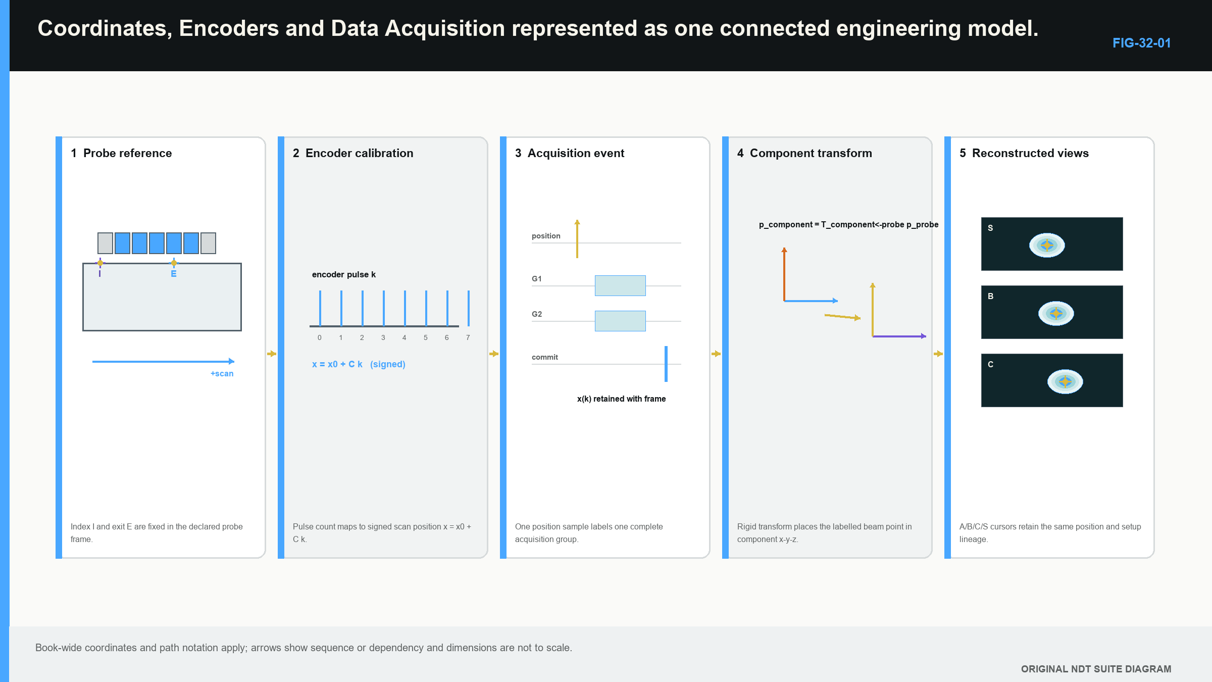
At each requested position, the instrument collects the complete enabled law sequence and stores the A-scans with the encoder coordinate. Repeating this process creates a line of position-tagged law groups. A B-scan can then place scan position along one axis. Corrected sector or other views can be linked to the same positions.
The encoder does not measure sound path or beam position; it measures movement at its sensing point. The setup applies a scale to convert counts into travel, a sign to set direction, a zero to set origin and an offset to connect the sensor or probe reference to the component datum.
This distinction explains several error patterns:
- wrong scale stretches or compresses the displayed length;
- reversed polarity mirrors movement along an axis;
- wrong zero or offset shifts every response by a similar amount;
- wheel slip creates local non-uniform position error;
- missed counts or triggers create gaps or irregular spacing.
Correct focal laws cannot repair an encoder error. A perfect encoder cannot repair an incorrect wedge offset or component geometry.
32.3 Encoder types and mechanical reality
A rotary incremental encoder produces counts as a shaft turns. The shaft may be connected to a wheel, axle, gear or chain. Two signal channels can also provide direction. High count density describes fine nominal resolution, but it does not guarantee that the wheel followed the component without slip.
Linear scales and cable-extension devices measure movement in other ways. Motor or drive encoders may report machine motion upstream of mechanical compliance. A scanner can report its axle accurately while the probe lifts, skews or lags behind.
Simple systems include one encoded wheel on a hand-guided probe. More controlled systems use guided carriages or two-axis scanners. A clicker arrangement encodes continuous scan travel and uses a deliberate event to advance the index line. Every additional axis needs its own scale, direction, reference and relationship to the component.
The following figure shows the measurement chain from encoder counts to component coordinates. The acoustic beam is linked only after the physical probe reference and focal-law geometry are included. [R014] [R042]
32.4 Understand scale, polarity, zero and repeatability
An encoder calibration compares indicated movement with a known physical distance. The study sequence is:
- Identify the encoder input and the physical axis it represents.
- Inspect the wheel, mount, cable, guide and contact surface.
- Establish a controlled start and end distance on a representative path.
- Zero at the start, move in the normal acquisition direction and compare the indicated travel.
- Apply the instrument's controlled scale correction if needed.
- Repeat the full distance, check intermediate points and return to zero.
- Check reverse direction when bidirectional travel will be used.
The physical meaning comes before the menu action. Scale sets distance per count. Polarity sets which direction increases the coordinate. Zero places the start. Repeated trials reveal slip, backlash or instability that one neat endpoint can hide.
Suppose a scanner travels a verified 360.0 mm while the display reports 354.6 mm. A candidate scale multiplier is 360.0/354.6, about 1.0152. After applying it, the important work is not admiring the corrected endpoint. Check 90, 180 and 270 mm, return to zero and repeat in both needed directions. Wandering intermediate values indicate a mechanical problem rather than a lack of decimal places.
No universal calibration distance is introduced here. The chosen distance must represent the intended movement and be long enough to expose important scale error under the applicable controlled requirement.
32.5 Encoder resolution and acquisition increment
Encoder resolution can be expressed as counts per millimetre or millimetres per count, and it states the nominal position-sensor step rather than position accuracy. A 0.05 mm count does not prove 0.05 mm accuracy when the wheel can slip or the reference offset is wrong.
The acquisition increment is the requested distance between stored complete law sets. It may contain several encoder counts. If resolution is 0.05 mm per count and the acquisition increment is 0.20 mm, a nominal stored position occurs every four counts.
Display pixel size is another separate quantity because software can interpolate extra pixels between stored positions. This may make an image smoother, but it does not add measured A-scans. Record the acquired spacing, not just the displayed grid.
Finer spacing gives more position samples and increases the required acquisition rate and file size. It does not narrow the beam or guarantee improved flaw sizing. Choose it from the demonstrated technique, target scale, scanner stability and rate capability.
32.6 Travel speed creates a required complete-set rate
The scanner moves a certain distance each second. The setup requires one complete enabled law set at each allowed distance increment. Their ratio gives the minimum rate of complete stored sets.
In words:
required complete-set rate = travel speed divided by maximum acquisition increment
| (32.1) Required complete-law-set acquisition rate · EQ-32-01 Where: f_required = required complete law sets per second (sets/s); v_scan = travel speed (mm/s); Delta_x = maximum permitted encoded increment (mm/set) Model limits: approximately steady travel; one valid complete enabled law set at each stored position; consistent distance units |
|---|
At 18 mm/s with a maximum increment of 0.6 mm, the system needs at least 18/0.6 = 30 complete law sets each second. Faster travel or finer spacing increases that demand.
The pulse repetition frequency, or PRF, counts pulse-receive cycles per second under the stated setup. If each law needs one sequential cycle, a simple ceiling for complete-set rate is PRF divided by the number of laws.
| (32.2) Idealised available complete-law-set rate · EQ-32-02 Where: f_available = ideal upper limit of complete law sets per second (sets/s); PRF = aggregate pulse-receive cycles per second (cycles/s); N_law = sequential firings required for one complete enabled set (cycles/set) Model limits: one firing per law; sequential execution; no allowance for receive-window, switching, averaging, processing, transfer or storage overhead; actual usable rate is measured on the configured system |
|---|
This is a planning ceiling, not a promised operating rate, because long receive ranges, several groups, averaging, processing and storage can reduce measured complete-set rate. Display refresh rate is also separate, and a screen can redraw smoothly while fewer complete positions are stored.
| Worked example · Connecting measured acquisition rate to position spacing WE-32-01 Given: A scanner moves at 100 mm/s. The configured system demonstrates 500 complete stored law sets per second. Encoder resolution is 0.05 mm per count. Find: The nominal distance between complete sets and the encoder counts per set. Method: Divide travel speed by measured complete-set rate. Delta_x = 100 mm/s / 500 sets/s = 0.20 mm/set counts per set = 0.20 mm / 0.05 mm per count = 4 Answer: Complete acquisitions are nominally 0.20 mm apart, or four encoder counts. What it means in practice: The arithmetic gives nominal spacing during steady valid travel. The actual record still needs checks for acceleration, slip, dropped triggers and overspeed. Common mistake: Using the screen refresh rate instead of the measured complete-law-set rate can make the calculated spacing fictional. |
|---|
32.7 Recognise overspeed and incomplete data
Overspeed occurs when travel demands complete positions faster than the configured system can provide them. Possible evidence includes an instrument warning, irregular position spacing, missing columns, incomplete law sets, too few positions for the travelled distance or a scan time that does not match the planned speed.
Compare expected and actual endpoints, position count and spacing. Check that each stored position contains the required groups and laws. Review coupling separately. Correctly encoded A-scans containing only coupling loss are still missing ultrasonic coverage even though their positions are complete.
Do not hide missing positions with interpolation. Generated pixels can make a gap look continuous without restoring acquired evidence. Reacquire the affected region with controlled overlap when the inspection plan permits it.
Acceleration matters near starts, stops and direction changes. A nominal average speed below the limit does not prove that every local movement stayed inside the rate capability. Guided scanning and sensible operating margin improve repeatability.
A short encoded trial from datum to stored data
Use a marked straight reference path 300 mm long. The probe reference mark begins at scan coordinate 0 mm and a fixed signed index offset from the weld centreline. The enabled setup requests one complete law set every 0.5 mm.
Before acquiring, move the scanner without ultrasound and compare its indicated position at 0, 100, 200 and 300 mm. Movement in the declared positive direction should increase the coordinate. Return to zero and note any failure to return or any difference between forward and reverse readings.
Next, collect a slow encoded pass over a stable reference reflector. At 0.5 mm spacing, a 300 mm acquired interval contains 601 positions when both endpoints are stored: the position at zero plus 600 half-millimetre steps. The exact system may handle endpoints differently, so compare the requested convention with the file rather than forcing the number.
Open several stored positions. Confirm that the complete required groups and laws exist at the start, middle and end. The linked A-scans should show the reference response rising and falling as the probe passes. A smooth B-scan alone cannot prove that every law is present.
Repeat at the intended operating speed. Compare stored position count, endpoint, elapsed time, overspeed status and coupling behaviour with the slow pass. If the fast dataset contains fewer positions, irregular gaps or missing laws, the configured rate or trigger handling is not supporting the proposed travel.
Now introduce a known coordinate feature, such as a marked target position. Check where the corrected display places it. If scan length is correct but the feature has one constant offset, review the probe reference and zero. If the whole length is stretched, review scale. If it is mirrored, review polarity.
This trial separates four controls that are often mixed together: encoder scale, component offset, complete-law-set rate and acoustic geometry. It also gives the learner a visible before-and-after record rather than a collection of menu values.
Position completeness and acoustic completeness
An encoded file can be position-complete and acoustically incomplete. Every requested coordinate may be present while the probe loses coupling across one band. The A-scans at those positions then contain little valid component response.
The opposite can also occur. Individual A-scans can contain good echoes, but the file can be position-incomplete because triggers were dropped. Both conditions create a coverage gap, but their causes and evidence differ.
Review position spacing and coupling indicators separately. A useful acquisition record shows where complete positions exist and where sound entered the component acceptably. Interpolation can fill neither missing law groups nor missing acoustic interaction.
Position records also need direction history. In a bidirectional raster, alternating lines may be stored with increasing component coordinates even though the scanner travels in opposite physical directions. Confirm how the software orders those samples. A reversed row on screen can be a display convention, a polarity fault or a real acquisition-order issue.
Use a known mark near both ends of the area when possible. One mark checks zero and local offset; two separated marks also challenge scale and direction. Their agreement does not prove every intermediate position, but disagreement immediately shows that a smooth image should not be trusted for length.
Preserve position units and origin in exported images. A strip labelled only with pixel numbers cannot be compared reliably with the component. The raw coordinate array or equivalent metadata remains part of the evidence even when the final reviewer sees only a linked view.
Keep the encoder's sensing point visible in the scanner sketch. This small detail explains why wheel lift, cable drag or frame movement can separate measured travel from probe travel. It also prevents a later reviewer from treating encoder counts as if they were direct measurements at the acoustic exit point.
32.8 Raster lines, direction and interruptions
A raster consists of neighbouring scan lines separated along the index axis. In a unidirectional raster, each acquired line travels in the same scan direction and the probe returns without acquiring. In a bidirectional raster, alternate lines travel in opposite directions.
Bidirectional acquisition can save movement time, but polarity, backlash, cable drag and probe response must remain acceptable in both directions. Index position must also be recorded or controlled. A one-axis encoder cannot independently prove the index value of each line.
For a simple area from index 0 to 64 mm in 8 mm steps, both boundaries are included at positions 0, 8, 16, 24, 32, 40, 48, 56 and 64 mm. That is nine acquired lines. Their acoustic coverage depends on verified beam width and overlap, not the line count alone.
When an obstacle interrupts a pass, stop at the last valid position and preserve the first segment. Re-establish the scanner from the datum, check offset, skew, scale and polarity, and begin the next segment with controlled overlap. Record any region that remains inaccessible. Dragging two images until they look connected is not a coordinate method.
Step up: more complex motion
Spiral, helical and multi-axis paths add changing orientation, surface geometry and coordinate transformations. The same foundations remain: every axis needs scale, sign, zero and a link to the component. Detailed cylindrical closure, robot tool-centre correction and rate budgeting are developed in the later acquisition-engineering chapters. They are not assessment dependencies for this Level 2 crossover.
In plain words
- Component coordinates begin at a recoverable physical datum.
- Scan, index and depth axes need declared positive directions and units.
- An encoder counts movement at its sensing point; it does not measure acoustic location.
- Scale, polarity, zero and offset create different position effects.
- Fine encoder resolution does not guarantee fine position accuracy.
- Travel speed divided by acquisition increment gives the required complete-set rate.
- PRF divided by law count is only an ideal planning ceiling.
- Missing or overspeed data cannot be repaired by smoothing the display.
Key terms
Datum; scan axis; index axis; depth; encoder; scale; polarity; offset; acquisition increment; complete-law-set rate; overspeed.
Key relationships
- encoder counts x distance per count -> indicated travel;
- indicated travel + sign + zero + physical offset -> component position;
- travel speed / permitted increment -> required complete-set rate;
- pulse-cycle rate / sequential law count -> ideal complete-set ceiling;
- measured complete-set rate + travel speed -> actual nominal spacing;
- valid positions + valid coupling + complete law groups -> usable encoded acquisition.
Common mix-ups
- Encoder resolution is not position accuracy.
- Encoder position is not acoustic beam position.
- Display refresh is not complete-law-set acquisition rate.
- A one-line encoder does not create a measured second coordinate.
- Correctly spaced empty A-scans do not prove ultrasonic coverage.
Bridge to Chapter 33
The setup can now form beams, arrange them into views and attach them to position. Chapter 33 shows how separate calibration checks establish time, distance, sensitivity and encoder relationships without pretending that one successful wizard proves them all.
Sources and further study
- [R014]
- [R042]
Study and revision only. This is not an approved inspection procedure, acceptance criterion or qualification.