
CHAPTER 6 · FMC / TFM / PCI Level 2
How TFM Forms an Image
In this chapter · 13 sections
Purpose
Total focusing method images can look immediately understandable, which creates the temptation to treat the display like a photograph. Every TFM pixel instead answers a calculated question: “If a reflector were at this coordinate, which sample from each transmit–receive A-scan would match that travel time, and what happens when those samples are combined?”
This chapter replaces “focused everywhere” with a model a technician can calculate, challenge and trace to raw evidence. It explains common delay-and-sum principles, not a manufacturer’s software.
Learning outcomes
After completing this chapter, the learner will be able to:
define a reconstruction grid in a declared component coordinate system;
calculate a simple transmitter–pixel–receiver travel time;
explain generic delay-and-sum TFM without claiming it is a proprietary algorithm;
describe how interpolation, RF sign, envelope, rectification and normalisation change the display;
trace an image response back to contributing elementary A-scans; and
identify the geometry, velocity, path and acquisition assumptions behind a reconstructed pixel.
Crossover map: from a focused beam to a pixel question
| Familiar UT/PAUT idea | TFM crossover |
|---|---|
| A conventional A-scan contains amplitude versus time. | Each FMC transmitter–receiver pair supplies an elementary A-scan from which a pixel-specific sample may be selected. |
| A PAUT focal law applies delays to form a beam for a chosen angle or focus. | TFM calculates a separate travel time for every transmitter, receiver and pixel, then aligns data during reconstruction. |
| Sound path is calculated from velocity and time. | The path model predicts time from the transmitter to the pixel and from the pixel to the receiver, including every material and mode on the route. |
| Probe index, wedge delay and component coordinates control location. | Element coordinates, wedge and surface models, ROI origin and encoder registration jointly control pixel location. |
| A focused beam has finite width and a target-dependent response. | A TFM point response also has finite width and side structure; small pixels do not remove that acoustic limitation. |
| An indication should be checked in the A-scan. | A TFM feature should be traceable to a coherent set of supporting elementary A-scans, not only a coloured region. |
The reconstruction grid
A two-dimensional TFM image normally begins with a region of interest, or ROI, divided into points or pixels. Before reconstruction, the technique must declare:
the component coordinate origin;
the positive scan, index and depth directions;
the location and orientation of the array elements;
the surface and wedge geometry;
the ROI start and end coordinates; and
the spacing between adjacent points in each direction.
The ROI is not acoustic coverage. Extending the box creates more calculations, not more sound. A point outside usable directivity, penetration or the qualified path remains unsupported even though software can colour it.
Each pixel must be registered to the same coordinate system as the probe and component. An encoder offset error moves the probe model relative to the component. A wrong wedge height changes the predicted interface crossing. A surface profile error changes both refraction and path length. These are not cosmetic setup issues; they change the sample selected from every contributing A-scan.
Travel time: the address of the sample
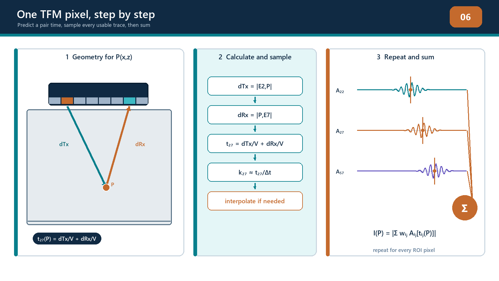
Consider a homogeneous isotropic component with no wedge for the moment. Element i transmits, element j receives, and the candidate pixel is at position r. For a selected transmit mode and receive mode, the travel time is the transmit distance divided by the transmit-mode velocity plus the receive distance divided by the receive-mode velocity.
tau_ij^(m-n)(r) = ||r - e_i|| / c_m + ||r - e_j|| / c_n
For a direct same-mode path, the two velocities are the same. For pulse-echo on one element, the two distances are also the same. Most FMC pairs, however, are pitch-catch pairs: the transmitter and receiver occupy different positions, so the route forms two sides of a triangle through the candidate pixel.
Points having the same total distance to a fixed transmitter and receiver form an ellipse in two dimensions. One A-scan sample is compatible with many points on that equal-time curve. A pixel becomes selective when many pair curves agree near the same coordinate under the correct path model.
Worked direct-path example
Assume the transmitter is at x = 0 mm, the receiver at x = 10 mm and both lie on z = 0 mm. A candidate pixel is at x = 6 mm, z = 20 mm. Using a single specimen velocity of 5.90 mm/µs:
transmit distance = √(6² + 20²) = 20.88 mm;
receive distance = √(4² + 20²) = 20.40 mm;
total distance = 41.28 mm; and
predicted travel time = 41.28 / 5.90 = 7.00 µs, approximately.
The reconstruction samples the i–j A-scan at about 7.00 µs, using the chosen interpolation method. A second pixel has a different predicted time. A second transmitter–receiver pair also has a different predicted time for the first pixel.
This calculation is deliberately simple. In a real angle-beam setup, the route may include wedge and specimen legs, refraction at the entry surface, a backwall reflection and a mode conversion. Every leg must be included. The familiar formula distance = velocity × time / 2 is not a universal shortcut for such a path.
Delay alignment and coherent summation
Suppose a real point-like reflector exists at the candidate pixel. Its echo reaches different receiver pairs at different times. Before alignment, the wave packets appear staggered. TFM uses the predicted time for each pair to select or shift the relevant sample. If the geometry and velocities are correct, the selected RF values have related phase and add constructively. Random noise and echoes from other locations are less likely to align across the full aperture.
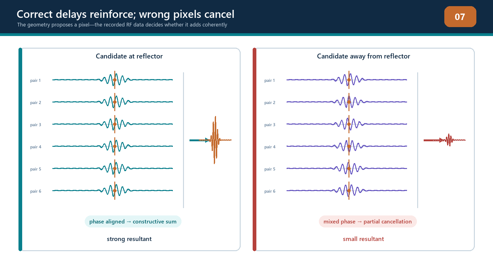
A generic amplitude reconstruction can be represented as a weighted sum of the selected samples.
I_P(r) = sum_i sum_j w_ij,P(r) s_ij(tau_ij,P(r))
This equation is a conceptual delay-and-sum model. It is not a statement of any commercial algorithm. The weight may account for aperture selection, apodisation, element directivity, transmission losses or another documented factor. Some implementations use all available pairs; others exclude channels, use sub-apertures or employ a reduced acquisition. Some sum real RF values and form an envelope afterwards. Other processing chains use analytic signals, frequency-domain methods or additional corrections.
The important sequence is:
choose a pixel and propagation path;
calculate a time for every included transmitter–receiver pair;
obtain the corresponding samples, normally with interpolation;
apply any declared weights;
combine them coherently; and
convert the result into the displayed quantity.
TFM does not transmit one physical beam focused at that pixel during an ordinary one-element-at-a-time FMC. The focus is synthesised from recorded pair data. “Focused at every point” means the calculation is repeated across the ROI.
Wedges, interfaces and general paths
For a wedge inspection, the element-to-pixel line cannot normally be treated as one straight specimen path. Travel time includes the route through the wedge, refraction at the entry surface and the route within the component. The entry point may differ for every element and pixel. A ray-tracing routine finds the path consistent with the geometry and the selected wave modes.
For a reflected or converted path, the general travel time is the sum of each leg length divided by that leg’s velocity.
tau_ij,P(r) = sum_(q in P_Tx) l_q / c_q + sum_(q in P_Rx) l_q / c_q
The model may include:
longitudinal propagation in the wedge;
longitudinal or transverse propagation in the component;
one or more reflections from known surfaces;
a conversion from one bulk-wave mode to another;
separate transmit and receive routes; and
different paths for different image views.
At every interface, the assumed crossing or reflection point must be physically possible. Ray tracing predicts travel time; it does not by itself prove that enough energy is transmitted, reflected, converted and received. An acoustically possible route can still have poor sensitivity because of element directivity, incidence angle, transmission coefficient, path length, attenuation or reflector orientation.
Interpolation and display processing
Calculated travel times rarely fall exactly on stored sample times. If the sampling interval is 0.02 µs and the required time is 7.01 µs, the processor must estimate a value between samples. Nearest-sample selection is simple but can produce position-dependent amplitude error. Linear, spline, sinc or frequency-domain interpolation can behave differently. The technician may not be able to choose the internal method, but should understand that sampling rate and interpolation influence peak stability and apparent position.
RF data contain positive and negative cycles. Common display routes are:
signed RF reconstruction: preserves oscillation and phase sign, so adjacent pixels may alternate positive and negative;
rectified display: removes or flips part of the signed waveform according to the stated rectification;
analytic-signal envelope: presents the magnitude associated with the reconstructed oscillatory signal; and
normalised image: scales values relative to a selected maximum or reference.
These routes are not interchangeable. An envelope changes the displayed quantity. Normalisation can make images with very different absolute responses look equally bright, and a colour map can increase visual contrast without improving signal-to-noise ratio. Record the processing chain before comparison.
The point-spread response
If a very small ideal reflector is reconstructed, it does not normally appear as one perfect pixel. It produces a point-spread response with finite axial and lateral extent and possibly side structure. Its form depends on frequency, bandwidth, aperture, element pitch and directivity, path geometry, view, interpolation and weighting. A real side-drilled hole, notch or pore adds its own scattering behaviour.
Therefore:
apparent image width is not automatically reflector width;
a narrower pixel pitch does not guarantee a narrower acoustic response;
two reflectors can be resolved only if their combined responses are sufficiently separable under a declared criterion; and
the same reflector may have different shapes in different views.
The point-spread response is the bridge to Chapter 8, where resolution and grid controls are examined in detail.
Field workflow: interrogating a TFM feature
When a feature appears in a TFM view, use the following sequence:
Confirm the dataset, encoded position, probe/wedge, component and reconstruction version.
Confirm the declared view and draw its transmit and receive paths.
Read the feature coordinate and check that it lies inside the qualified ROI and covered volume.
Display representative supporting A-scans across several transmitter and receiver positions.
Compare observed arrival times with the times predicted for the pixel.
Check whether RF cycles align after the same delays used by the reconstruction.
Look for clipping, dead channels, cross-talk, ring-down or coupling changes.
Change only one reconstruction assumption at a time—such as velocity, surface or path—and observe whether the feature moves or defocuses as predicted.
Compare a complementary valid view or conventional PAUT/UT evidence.
Record uncertainty and stop if the feature depends on an unverified model or processing setting.
This does not mean every production indication must be manually recalculated. It means the technician must be able to audit representative features and challenge unexpected ones.
Practical 6 — Build two TFM pixels by hand
Aim
Calculate and manually combine samples for two candidate pixels, then compare the result with a vendor-neutral software reconstruction and the elementary waveforms.
Resources
a controlled FMC teaching dataset from a homogeneous block containing a known small reflector;
declared element coordinates, specimen velocity, sample interval and time zero;
a worksheet or spreadsheet that does not conceal the travel-time formula;
reconstruction software capable of displaying the same direct path; and
a saved reference image and channel-health record.
Method
Verify dataset identity, matrix completeness, active elements, time zero and velocity.
Select four widely distributed transmitter–receiver pairs, including one pulse-echo diagonal pair and three pitch-catch pairs.
Define Pixel A at the known reflector coordinate and Pixel B at a nearby background coordinate.
Calculate the transmit distance, receive distance and total travel time for each pair and pixel.
Convert each time to a sample index. Record the fractional index rather than rounding silently.
Extract the nearest sample and a linearly interpolated sample. Retain both results.
Plot the four A-scans before alignment, then shift them to place each pixel’s predicted time at a common origin.
Add the selected signed samples for Pixel A and Pixel B. Note which pairs contribute constructively and which do not.
Reconstruct the ROI using the declared software path and compare the relative Pixel A and B responses.
Open at least eight additional supporting A-scans around the aperture to confirm that the observed behaviour is not caused by one dominant or faulty channel.
Evidence to retain
completed travel-time table with units;
source element and pixel coordinates;
selected A-scan plots before and after alignment;
nearest-sample and interpolated sums;
screenshot or export of the software reconstruction with settings;
a short explanation of discrepancies; and
instructor sign-off that the path and coordinate system were used correctly.
Stop rules
Stop and escalate if the dataset identity or velocity is unknown; the sample time origin cannot be established; any selected channel is clipped or missing without an authorised exclusion; the software path cannot be matched to the manual path; or Pixel A’s calculated arrival falls outside the recorded time range. Do not adjust velocity or coordinates merely to force agreement with the displayed image.
Common traps
Calling FMC “TFM data” without separating acquisition from reconstruction.
Dividing time by two for an asymmetric pitch-catch or multi-leg path.
Treating the centre of a coloured blob as an independently measured coordinate.
Assuming the ROI boundary is the coverage boundary.
Comparing a signed RF pixel with an enveloped or normalised pixel as though the units were identical.
Rounding travel times to whole samples and ignoring interpolation error.
Believing a high summed response proves the selected path is the true path.
Hiding a model mismatch by changing velocity until the image looks tidy.
Reporting pixel pitch as sizing accuracy.
Inspecting only the final image and never the elementary A-scans.
Chapter summary
TFM is a reconstruction, not a photograph and not a physical beam focused everywhere at once. The processor defines a grid, predicts a transmitter–pixel–receiver time for every included pair, samples the elementary A-scans, aligns the contributions and forms a displayed value. Accurate reconstruction depends on declared coordinates, element positions, velocities, geometry and propagation paths. Wedges, refraction, reflections and conversions add legs that must be modelled explicitly.
When the model is correct, a real event can align across many pairs. When it is wrong, valid energy can defocus or unrelated energy can be placed misleadingly. Interpolation, RF/envelope processing, weighting and normalisation further influence the displayed pixel. A competent technician can trace a response back to supporting A-scans, state the assumptions and stop when the model cannot be defended.
Study and revision only. This is not an approved inspection procedure, acceptance criterion or qualification.