From One Conventional Probe to One Phased-Array Beam

Why this matters

Phased-array ultrasonic testing can look like a completely different method when the first screen is a coloured sector. It is not. The same pulse still enters the component, meets boundaries and returns as echoes. The important change is in the probe. A conventional probe usually uses one active piece of material at a time. A phased-array probe divides that active material into small elements that can be timed separately. This chapter builds the change one step at a time, beginning with the conventional A-scan already familiar from UT and ending with one focal law that creates one beam.

What you already need

• The pulse-echo journey from instrument to probe, component and back.
• The difference between echo time and echo amplitude on an A-scan.
• The basic meaning of sound path, wave mode, refraction and gain.
• The habit of separating an indication from its possible cause.

What you will learn

• State what remains unchanged when moving from conventional UT to PAUT.
• Follow the change from one conventional crystal to one array element and then many elements.
• Explain how small time delays change the direction or focus of a combined beam.
• Distinguish an element, an active aperture and a focal law.
• Trace one PAUT firing from the pulser to its stored A-scan.
• Recognise what a first sector display adds and what it does not prove.

Words you will meet

• Element: one individually addressable part of an array probe.
• Array: a probe containing several elements in a known arrangement.
• Aperture: the selected elements used together for one transmit or receive event.
• Delay: a small timing difference applied to an element.
• Focal law: the element selection and timing used to make one defined beam condition.
• Law group: a related set of focal laws used for one examination purpose.
• Sector display: a view that places responses from several beam angles beside one another.

27.1 Begin with the conventional UT picture

Place a conventional angle-beam probe on a steel test piece. The instrument sends an electrical pulse through the cable. The probe changes it into an ultrasonic pulse. The wedge guides the pulse toward the entry surface, refraction establishes the wave mode and direction in the steel, and the sound travels through the component. A returning echo reaches the probe and becomes an electrical signal. The instrument then shows an A-scan.

That chain remains the foundation of PAUT. Material velocity still affects position. Wave mode still matters. Surface condition and couplant still affect transmission. Attenuation, grain structure and reflector orientation still change the received response. A back-wall corner can still produce a strong geometric echo, while a poorly oriented planar discontinuity can return little energy. PAUT does not repeal any of that physics. [R014] [R016]

Imagine that the conventional probe is held still while the examiner changes the selected angle by replacing the probe or wedge. Each arrangement produces a new A-scan from a different direction. The examiner may need several placements to examine a weld volume. Phased array aims to create several useful beam conditions from one array and wedge assembly. It does this electronically, but the result of each firing is still an ultrasonic waveform.

This point is worth holding onto when the screen becomes busy. A coloured sector is not a photograph. It is a presentation made from several A-scans whose positions depend on the entered probe, wedge, material and focal-law information. The most reliable route into PAUT is therefore to understand one A-scan first and add the electronic changes in order.

27.2 Replace one crystal with one array element

A conventional single-element probe contains one main active area. An array probe divides a larger active area into smaller pieces called elements. Each element can be connected to a pulser and receiver channel under instrument control. The elements are arranged in a known order, often as a straight row in a linear array.

Start by selecting only one array element. Pulse it by itself and receive on it by itself. The result is not yet the powerful beam normally associated with PAUT. It is simply a very small ultrasonic source and receiver. Its pulse still travels through the wedge and component, and its returning signal can still be shown as an A-scan.

This single-element thought experiment removes much of the mystery. An element is not a complete sector, an angle or an image pixel. It is one physical part of the probe. The instrument needs to know which element it is addressing, where that element sits, and how its signal is connected. If element numbering or connector mapping is wrong, the instrument may time the wrong physical positions while continuing to draw a tidy display.

One small element usually spreads sound over a relatively broad angular range in the plane of the array. That usable angular range is called its directivity. Directivity helps later elements contribute to a steered beam, but it also limits how far the array can steer efficiently. The detailed field calculation belongs in Part V. At this stage, picture each element as a small source with a finite spread, not as a laser line.

27.3 Select several elements: the active aperture

Now select several neighbouring elements and fire them together. The selected group is the active transmit aperture. If the same elements listen for the echo, they form the receive aperture as well. Some systems can use different transmit and receive selections, so the complete law record must identify both when they differ.

When neighbouring elements vibrate at the same time, their sound fields overlap. In some directions the pressure contributions reinforce each other. In other directions they partly cancel. The combined field has a more useful main direction than the field from one small element. Increasing the aperture can change sensitivity, beam width, focus and the range over which the beam behaves as intended.

The aperture is a selection, not the whole probe. A 64-element probe might use elements 1 to 16 for one firing, 2 to 17 for another, or a different number of elements for another purpose. The full physical array, the selected active elements and the effective acoustic width must not be treated as the same quantity. Chapter 29 develops that distinction.

The instrument also has hardware limits. A probe may contain more elements than the instrument can pulse or receive at once. Multiplexing connects the available electronics to different element addresses in an organised sequence. For a Level 2 reader, the practical lesson is simple: a probe label does not prove that every proposed aperture can be used. The enabled instrument, connector, probe and software combination decides what can actually fire.

27.4 Add small delays to change the beam

If every selected element fires together, the combined wavefront tends to travel in the natural direction set by the aperture and wedge. If one element fires slightly before its neighbour, and the next fires slightly later again, the small wavelets meet in a different pattern. Their strongest reinforcement can be tilted. This is electronic steering.

The delays are very short, commonly fractions of a microsecond. Their physical meaning is more important than their size. Timing lets sound from elements at different positions arrive together along a chosen direction. The instrument is not bending a finished beam after it leaves the probe. It is arranging when the separate contributions begin so that a combined wavefront forms.

A different delay pattern can make contributions arrive together near a selected point. This is electronic focusing. Steering mainly changes the beam direction. Focusing aims to improve concentration around a selected region. A law can include both effects. The focus is not a pin point that remains equally sharp everywhere; the useful focused region has finite width and length.

The wedge and interface remain part of the calculation. Each element has a different path through the wedge. Refraction then changes direction at the component surface. A delay pattern that would work in one wedge material or component velocity may be wrong in another. Correct probe geometry, wedge data, material velocity and wave mode are therefore inputs to the timing, not details to be patched later with gain.

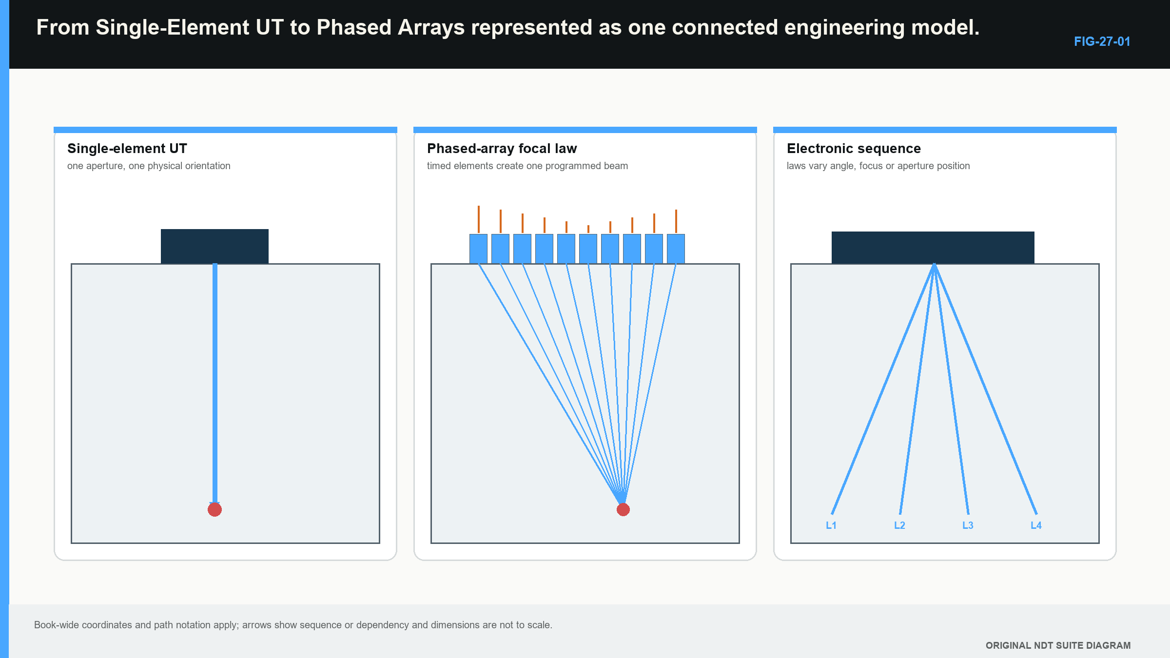
The three-panel progression is now complete:

1. One selected element produces a broad small-source response.
2. Several elements used together form an aperture with a combined field.
3. Controlled delays change where the contributions reinforce, altering direction and focus.

The following figure connects these three stages. Read it from left to right before looking at the sector-style presentation on the far side. [R014] [R046]

27.5 One focal law creates one beam condition

A focal law is the complete instruction for one beam condition. At minimum, it identifies the participating transmit and receive elements and the delays applied to them. The enabled setup also connects that law to a wave mode, intended angle, focus description, time range, gain treatment and geometric model.

It is tempting to call a focal law “one angle.” That is incomplete. Two laws can share a nominal angle but use different aperture positions or focal depths. Two laws can use the same selected elements but different delays. A law therefore describes a configured transmit-receive event, not just the number printed beside a ray.

Follow one law through the system:

1. The setup selects the law and its element addresses.
2. The pulser sends the programmed excitation to the selected elements at their stated delays.
3. The element contributions pass through the wedge and enter the component.
4. The field interacts with material, geometry and any discontinuity.
5. Returning sound reaches the selected receive elements at different times.
6. Receive delays align the signal portions predicted to belong to that beam condition.
7. The instrument combines the channel signals into one receive waveform.
8. Gain, filtering and digitisation create a stored or measured A-scan.

The combined A-scan still has time or distance horizontally and response amplitude vertically. It can be inspected like a conventional trace, provided the reviewer also knows which law produced it. A response at a certain time is not automatically at the displayed corrected point. That location depends on the law, wedge path, velocity and coordinate model.

One law can be useful by itself. For example, an array can reproduce a fixed-angle beam using one aperture and one delay pattern. The practical comparison with conventional UT is then direct: both methods create a pulse, receive an echo and show an A-scan; the array method creates the beam by coordinating several small elements.

A guided crossover from one conventional shot to one array law

Picture a conventional 45-degree probe placed beside a weld. The examiner adjusts range and gain, moves the probe until a reference echo peaks and reads the A-scan. The beam direction comes mainly from probe and wedge construction. Repeating the test at another angle normally requires another probe, wedge or position.

Now place an array on a suitable wedge at the same region. Select one aperture and one focal law intended to create a comparable beam. The array instrument fires several elements at slightly different times, combines the received element signals and presents one A-scan. The examiner can still maximise the same reference echo, read its time and compare its response. The familiar evidence has not disappeared.

The new information is the law identity. The record now needs the selected element addresses, their aperture position, the law timing basis and the wedge/material model that gives the beam its nominal direction. If a later law uses a different aperture or angle, it produces another A-scan with another physical sensitivity.

This comparison also shows what not to compare casually. A conventional probe and an array law may share a nominal refracted angle while differing in aperture, frequency response, beam width and focus. Similar centre lines do not make their responses interchangeable. Use a common reference feature and the actual configured systems when examining the crossover.

27.6 From one law to a related law group

The advantage of PAUT becomes more visible when the instrument runs several related laws in sequence. One group might change angle while keeping the aperture near one position. Another might move the active aperture along the array while keeping angle and focus similar. A third might use different focal depths. These sequences are developed in Chapter 31.

Each law produces its own A-scan. If a group contains 31 laws, one complete pass through that group contains 31 transmit-receive events unless the implementation combines or repeats firings in another declared way. The instrument can arrange the resulting traces by law order and sound path to create a sector-style view. That view helps the examiner compare responses across beam conditions.

The display can make the group feel simultaneous. Physically, many systems fire the laws in a rapid sequence. More laws take more pulse-receive cycles, which affects the rate at which complete groups can be collected. This matters during encoded scanning because the scanner must not travel so far that required positions are skipped. The rate calculations are deliberately postponed until Chapter 32, after law groups, displays and encoding have concrete meaning.

Groups should be named by purpose, not by visual excitement. A sectorial group may examine several weld-face orientations. A fixed-angle stepped-aperture group may cover adjacent lateral positions. A straight-beam group may monitor coupling or parent material. The presence of more groups does not by itself improve coverage. Every group uses time, storage and review effort.

27.7 What PAUT changes, and what stays the same

PAUT can provide several practical benefits. Multiple angles can be produced without swapping probes for every direction. An aperture can move electronically across part of the array. A selected region can be focused. Encoded data can preserve response changes along the component. Linked displays can help a reviewer connect the underlying A-scan with position and law.

The method also adds controls. The setup needs correct probe and wedge data, element order, aperture selection, delays, angle and focus definitions. It needs an acquisition plan that accounts for law count, range and travel. Array condition matters because a dead or weak element can change the beam while an image still looks plausible. Steering and focusing can also produce side or grating responses that a centreline ray does not show.

None of those controls replaces conventional reasoning. The examiner still asks whether the echo is repeatable, whether the sound path is plausible, whether geometry could explain it, whether the required volume was covered and whether the data quality supports interpretation. Calibration still establishes particular relationships rather than blessing the whole inspection with one green tick.

The safest mental model has four layers:

• Physics: how sound travels and interacts in the component.
• Beam control: which elements and delays create each law.
• Acquisition: how laws are sequenced, positioned, measured and stored.
• Interpretation: how waveforms and views support a restrained conclusion.

When something looks wrong, locate the layer before changing controls. A wrong material velocity is not fixed by colour palette. A reversed encoder is not fixed by wedge delay. A weak angle at the edge of an array's useful range is not made valid by increasing its displayed brightness.

27.8 A short history, and the next practical step

Industrial ultrasonic testing developed through early transmission and pulse-echo instruments, improved piezoelectric transducers, portable electronics and digital acquisition. Arrays became practical when instruments could control many channels and small delays reliably. This history explains why PAUT retains conventional pulse-echo language while adding terms from electronics and imaging. [R060]

The history is useful context, but it is not needed to operate the learning model. The important crossover is physical: one conventional active area becomes several separately addressable elements; selected elements form an aperture; delays create one focal law; several laws form a purposeful group; and every firing still produces ultrasonic evidence that can be traced back to an A-scan.

The next chapter begins with those A-scans and asks how the same reflector appears when the data are arranged in different views. Digitisation and file structure are kept behind the display at first. That order makes the screen a representation of known echoes, not a collection of unexplained coloured shapes.

In plain words

• PAUT keeps the pulse-echo physics learned in conventional UT.
• One array element is one small physical source and receiver, not an image or an angle.
• Several selected elements form an aperture.
• Small timing differences make element contributions reinforce in a chosen direction or region.
• One focal law defines one transmit-receive beam condition.
• A law group runs related focal laws for one examination purpose.
• Each law still produces a waveform that can be inspected as an A-scan.
• A sector display helps compare laws, but it does not prove beam quality, coverage or reflector type.

Key terms

Element; array; active aperture; delay; focal law; receive law; law group; sector display; multiplexing.

Key relationships

• conventional pulse-echo foundation + individually timed elements = phased-array beam control;
• selected elements + delay pattern = one focal law;
• related focal laws + execution order = one law group;
• one law firing + received channel combination = one underlying A-scan;
• more laws + finite pulse-receive time = lower possible complete-group rate.

Common mix-ups

• The complete probe is not the same as the selected aperture.
• A focal law is more than a nominal angle.
• Steering changes the combined field; it does not bend an already formed ray.
• A sector picture is assembled from waveforms; it is not a direct photograph.
• Gain can alter display height, but it cannot repair wrong timing, geometry or coverage.

Bridge to Chapter 28

Chapter 28 keeps one reflector in view while the data presentation changes. It begins with the A-scan, then builds the S-, B-, C- and D-type views. Only after those views make sense does it introduce the digitisation choices that sit underneath them.

Sources and further study

• [R014]
• [R016]
• [R046]
• [R060]