Proving the Data, Model and Technique

Why this matters

An advanced image can remain attractive while a receiver column is weak, velocity is wrong or a geometry echo is reconstructed as a target. One check cannot prove all three layers; the dataset must first be healthy. The propagation and reconstruction model must then place known events correctly. Finally, the complete technique must demonstrate its assigned task on representative targets. When an unexpected feature appears, a controlled diagnostic changes one suspected cause at a time and preserves the first anomalous state.

What you already need

• FMC matrix-health and acquisition-integrity checks from Chapters 47 and 48.
• One-pixel travel-time and path reasoning from Chapters 49 and 50.
• Reconstruction-control and PCI limits from Chapters 51 and 52.
• Familiar PAUT equipment, reference-target and encoder checks.
• The distinction between a symptom, a likely cause and confirming evidence.

What you will learn

• Apply three separate proof gates to a matrix-imaging technique.
• Distinguish equipment health from reconstruction correctness and application performance.
• Classify artefacts by acquisition, model, propagation, reconstruction, display and position source.
• Use a symptom-to-hypothesis-to-challenge diagnostic sequence.
• Estimate the location scale of a small direct-path timing error.
• Decide when controlled reprocessing, reacquisition or escalation is required.

Words you will meet

• Verification: check that an identified system or model behaves as specified for a defined test.
• Performance demonstration: evidence that the complete technique performs its intended task under represented conditions.
• Artefact: displayed structure caused or placed by something other than the claimed target interpretation.
• Hypothesis: one possible explanation retained for testing.
• Discriminating check: observation expected to differ between competing explanations.
• Quarantine: controlled hold preventing uncertain data from being reported or altered.
• Root cause: best-supported originating cause after evidence-based testing.

53.1 Use three proof questions in order

The first proof concerns the acquired dataset; the identified instrument, probe, wedge, channels, encoder and stored records must operate inside their defined health limits. This includes timing, noise, clipping, element activity, pair completeness and file identity. The second proof concerns the model and reconstruction. Known events must be placed at correct times and component coordinates using the declared velocity, wedge, surface, element map, paths, ROI, pair set and software version.

The third proof concerns the application. Representative targets must demonstrate the required detection, location, separation or sizing task throughout the intended domain; a central side-drilled hole cannot establish every weld orientation, edge region or tip-sizing claim. Research and implementation guidance for matrix imaging uses the same separation because equipment condition, reconstruction fidelity and application capability answer different questions. Artefact studies also show that changes in acquisition, model or display can produce similar-looking symptoms. [R027] [R028] [R045] [R061]

The figure below turns the three proofs into a ladder; a later gate does not repair a failed earlier one.

The learner should notice that every later claim depends on the gate below it. A polished image cannot repair an incomplete matrix or an incorrect coordinate model.

53.2 Gate A checks the acquired system

Gate A asks whether the connected system produced a trustworthy source record; the check includes instrument, probe, wedge, cables, element map, scanner interfaces and the software configuration controlling acquisition. It inspects transmit rows and receive columns so the two channel roles are visible. A dead transmitter can weaken one row; a receiver failure can weaken one column. One isolated file defect can affect a cell. Timing spread can reduce coherence without making any channel appear dead; a reconstructed image may hide these losses because remaining pairs still form a smooth feature.

The health record can include relative element response, arrival consistency, receiver noise, clipping state, cross-talk, sample range, matrix dimensions, encoder behaviour and file write success. It uses declared reference data and tolerances from the controlled technique or applicable equipment requirement. Passing Gate A means the system met the defined health checks. It does not prove that a selected TFM view covers a weld or that PCI can size a crack.

53.3 Gate B checks time, path and coordinates

Gate B uses known targets at more than one depth and lateral position. It confirms probe and wedge identity, element coordinates, material speed, component thickness, surface model, time origin, encoder zero and sign, path labels, ROI, aperture, grid and reconstruction version. A common time offset can move many responses similarly. Wrong velocity often produces a displacement that grows with path length; a wrong surface can create position-dependent error. Reversed encoder direction mirrors scan position while a local cross-section may still look believable. Several targets help separate these patterns.

For amplitude TFM, the check can include fixed-scale response stability as a target moves relative to the grid and reference response where the approved technique uses it. For PCI, it verifies repeatable detection, position and expected target behaviour in that implementation; it does not invent a universal decibel equivalence or coherence tolerance. Passing Gate B means the controlled inputs map the selected known events acceptably; it does not establish performance on every production reflector.

53.4 Gate C checks the complete application

Gate C uses representative material, geometry and target behaviour. For a weld-like task, targets can include shallow, mid-wall and backwall-adjacent positions; planar and tip-like features; volumetric response; and relevant root, cap or sidewall geometry. Every reported path and image domain is challenged in its weakest region. Material attenuation, scattering, surface transfer, encoded coverage and scanner repeatability are represented. Detection, location, target separation and sizing are tested separately when the technique claims them.

Performance belongs to the demonstrated range of component thickness, material, probe, wedge, matrix scheme, paths, processing and operator conditions. A result on thin flat carbon steel does not transfer automatically to a thicker curved clad component. The targets need truth records. Machined reflectors give known geometry and repeatability but may not reproduce natural crack scattering. Representative natural or implanted targets provide other evidence while adding truth uncertainty. The demonstration statement names what each target supports.

53.5 Give every check a source and action

A verification record states the identified system, software revision, reference specimen and target, measured value, unit, tolerance, source of tolerance, pass or fail, corrective action and repeated result. Screen pixel spacing and operator habit are not tolerance sources.

Organisations and standards can use calibration, standardisation and verification differently. The Level 2 learner follows the controlled terminology while retaining the functional distinction among health, mapping accuracy and application performance.

Encoder verification uses an independent length reference and checks zero, sign, units, scale and return behaviour. A trial at intended speed compares physical travel with stored positions and looks for repeated frames, gaps and abrupt jumps. Absence of an instrument alarm does not prove continuity.

Re-verification occurs at the intervals and triggers defined by the procedure. Typical triggers include probe or wedge change, cable or scanner change, temperature shift, matrix or aperture change, gain or filter change, geometry or velocity change, path or ROI change, software update and unexpected reference behaviour.

When a post-use check fails, affected production data are quarantined back to the last valid check. Correction is followed by the failed check and every dependent check. Earlier data receive an authorised disposition rather than an optimistic assumption.

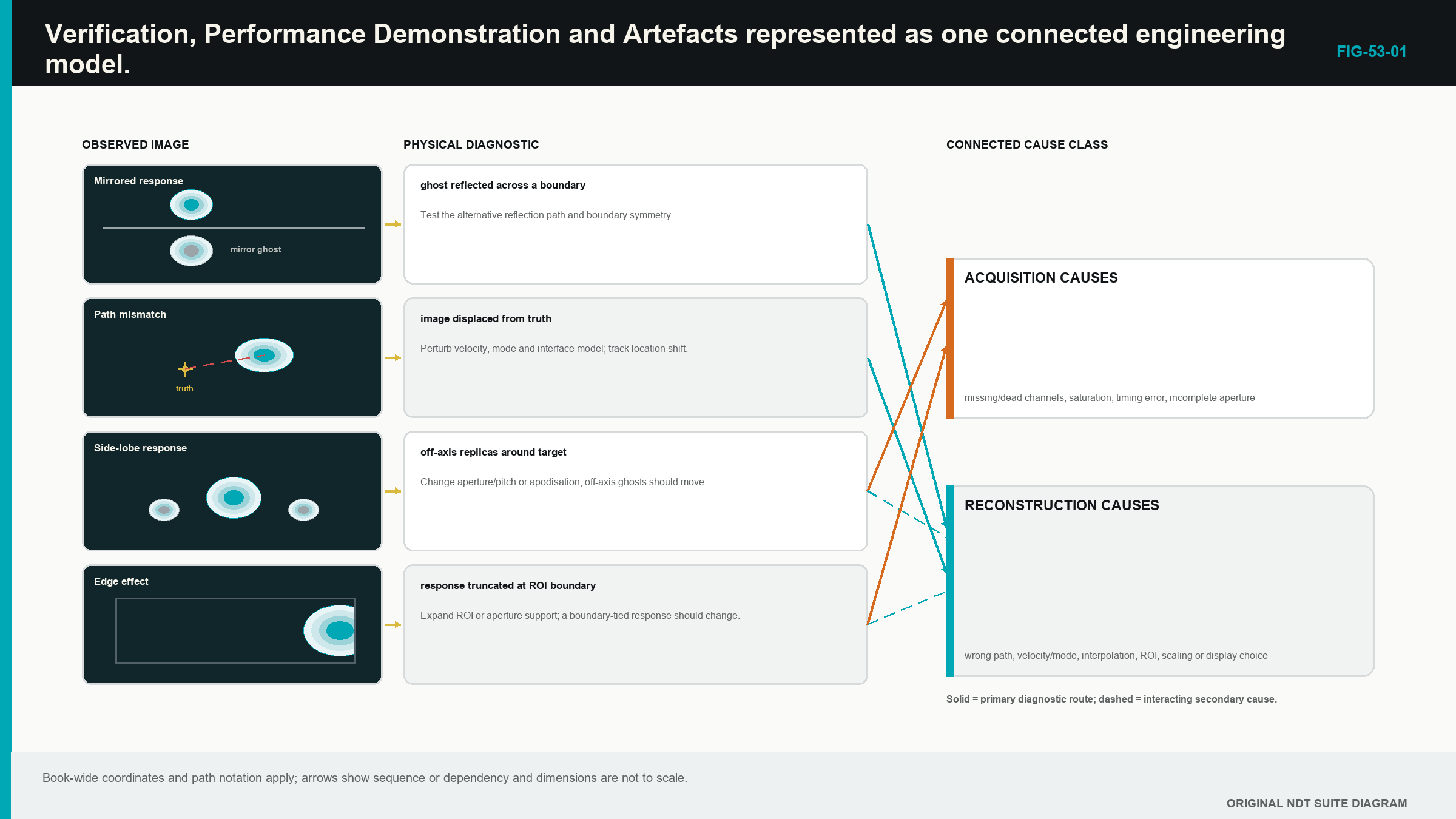
53.6 Classify an artefact before changing controls

An acquisition source includes coupling, clipping, weak channels, missing traces, filtering, short time range or cross-talk. A geometry or model source includes wrong velocity, wedge, surface, thickness, element position, time origin or coordinate registration.

A propagation source includes unintended mode, reflection, multiple, reverberation, side lobe, grating lobe, shadow or real geometry echo. A reconstruction source includes wrong path, pair set, aperture, ROI, grid, interpolation, weight or normalisation.

A display source includes envelope route, threshold, palette, smoothing and resampling. A position or governance source includes encoder slip, wrong component file, mismatched setup, repeated frame, software-version mismatch or incomplete transfer.

One symptom can have several sources. A weak area can be coupling loss, attenuation, directivity or threshold. A duplicated feature can be a multiple, a lobe, repeated encoder positions or file assembly error. Classification keeps competing explanations visible long enough to test them.

The initial dataset and image are copied and protected before any slider moves. Preserving the first anomalous state prevents a correction from erasing the evidence needed to identify cause.

53.7 Follow symptom, hypothesis, prediction and challenge

First describe the symptom without naming a cause. State its component coordinates, view, scale, scan range and repeatability. Then inspect raw A-scans, matrix health, coupling and encoder history.

Next draw the reported path and at least one competing path. List two or more hypotheses from different source classes. Choose one discriminating check whose expected result differs between them. Record those predictions before performing the check.

Change one controlled variable on a working copy. If wrong velocity is suspected, predict how known targets at different depths should move. If a lobe is suspected, alter aperture within a demonstrated diagnostic range and predict how the duplicate changes relative to the main response. If encoder slip is suspected, inspect stored coordinates and physical marks without modifying reconstruction.

Compare with known-good data using fixed displays. Record the best-supported root cause, the affected claims and the authorised corrective route. A diagnostic setting outside production limits remains labelled non-reportable even when it exposes the cause.

53.8 Recognise acquisition and position signatures

A weak transmit row or receive column can create directionally structured loss. An authorised exclusion changes effective aperture and must already sit inside demonstrated performance. Silent removal is not a repair.

Clipping flattens RF and changes phase. Low gain or penetration leaves phase controlled by noise. Neither is corrected through display gain. Lost coupling often affects many pairs at the same encoded position. A dedicated coupling signal and repeat scan distinguish it from a real attenuation zone.

Fixed-time cross-talk follows instrument timing across pairs. After reconstruction it can appear as a curve or line. Changing component path or probe lift may leave the electronic time fixed, providing a useful challenge.

Encoder dropout stretches, compresses, repeats or interrupts features along scan. The stored position sequence and independent travel distance are the direct evidence. Reconstructing again cannot create missing physical positions.

53.9 Recognise model, path and display signatures

Wrong velocity, time origin or wedge delay changes predicted sample addresses. Several known targets reveal whether the error is common, path-length dependent or position dependent. Changing an ROI offset to make one target align can hide the real model error.

Curvature and local surface preparation can shift interface points. A flat model on a curved surface often creates lateral variation in depth and focus. The remedy is an authorised surface model or new evidence, not a cosmetic image translation.

Real backwall, root, cap, counterbore and attachment energy can reconstruct under unintended paths. Draw the travel route and compare raw time. Path degeneracy requires a materially different view or independent geometry; one bright reconstruction cannot choose between equal-time causes.

A coarse grid can miss a peak. An ROI edge can cut a response. Smoothing can join features. Independent normalisation can make a noise-only view colourful. Fixed-scale baseline images expose these display and reconstruction changes.

For PCI, coherent geometry and cross-talk can appear strong, while a valid specular face can be weak. When amplitude and coherence disagree, compare source signal range, target scattering, aperture, band, masks and the representative-target evidence before deciding what the disagreement means.

53.10 Choose reprocessing, reacquisition or escalation

Controlled reprocessing can be valid when the original acquisition is complete, linear, correctly positioned and long enough, and the correction changes an authorised reconstruction input. Examples include a corrected supported velocity, ROI boundary or display setting applied to a protected copy.

Reacquisition is normally required for clipping, insufficient useful signal, wrong analogue filtering, unstable coupling, missing time, excessive missing channels, encoder gaps or the wrong physical scan route. The evidence needed for the result never survived.

Escalation is required when root cause remains uncertain, a proposed correction changes an essential variable outside range, a new path or algorithm is needed, application capability becomes uncertain or the result can affect acceptance without a controlled disposition.

The decision is tied to claims. A display correction can leave detection and location evidence unchanged. A velocity correction changes location and possibly coherence. An aperture exclusion can change sensitivity, resolution and sizing. The report and review scope follow those affected outputs.

53.11 Calculate the scale of a timing error

For a small timing offset in a direct homogeneous pulse-echo path, the one-way location scale is half the speed multiplied by the round-trip timing error. The relationship gives a useful diagnostic magnitude before more complex paths are considered.

53.12 A completed diagnostic case

A known target appears mirrored along the scan axis, while its local depth and shape look normal. Gate A matrix and timing checks pass. Gate B shows correct depth at two reference positions but stored encoder values decrease while the probe physically moves in the declared positive direction.

Two hypotheses are retained: reversed encoder sign and an image-display mirror. A raw position export predicts decreasing coordinates only for the encoder hypothesis. The export confirms that pattern. The controlled sign is restored, encoder distance and direction are reverified, and dependent coordinate checks are repeated.

The affected production scan is not repaired by flipping a screenshot. Its matrices were attached to reversed positions under the source record. The authorised process determines whether the position mapping can be corrected from complete trustworthy encoder data or whether reacquisition is required. The original anomalous dataset remains quarantined and preserved.

This case illustrates the full method: separate proof gates, describe the symptom, keep alternatives, choose a discriminating check, correct one cause and assess data impact.

Step up

Chapter 61 develops validation and reliability evidence for Level 3 matrix techniques. Chapter 62 extends the diagnostic ladder into dataset forensics and reproducible experiments. Chapters 69, 72 and 80 provide engineering detail for timing, coherence artefacts and software-system integrity.

In plain words

• Dataset health, reconstruction correctness and application performance are separate proof gates.
• Passing an element check does not prove weld coverage or sizing capability.
• Artefacts can begin in acquisition, modelling, propagation, reconstruction, display or position control.
• The first anomalous state should be preserved before diagnostic changes.
• Competing hypotheses are tested with a check expected to produce different outcomes.
• One variable changes at a time on a controlled copy.
• Reprocessing needs complete valid source data; missing or distorted acquisition often needs a new scan.
• Unresolved or out-of-range changes require authorised technical review.

Key terms

• Verification: evidence that a defined item meets a stated check.
• Performance demonstration: evidence for the complete assigned task in represented conditions.
• Artefact: image structure not supporting the claimed target interpretation.
• Hypothesis: retained possible cause.
• Discriminating check: test that separates competing causes.
• Quarantine: controlled hold on uncertain data.
• Root cause: originating cause best supported after testing.

Key relationships

• Gate A -> Gate B -> Gate C: health precedes mapping correctness, which precedes application claim.
• symptom -> hypotheses -> predicted check -> evidence: controlled diagnosis avoids slider-driven guessing.
• Delta_r ~= c Delta_t/2: direct-path timing error provides a first location-shift scale.
• fault class -> affected claims -> disposition: corrective scope follows what the fault can change.

Common mix-ups

• Equipment health is not application qualification.
• One correctly located target does not validate a whole ROI or every path.
• A coherent feature is not automatically a relevant discontinuity.
• A diagnostic improvement on an uncontrolled copy is not a reportable correction.
• Correcting a display cannot repair missing or clipped source data.

Bridge to Chapter 54

Chapter 53 established whether the evidence is fit to interpret. Chapter 54 now completes the Level 2 crossover. It separates detection, location, characterisation, sizing and evaluation, then preserves the source data and reconstruction recipe so another authorised reviewer can reproduce the conclusion.

Sources and further study

• [R027]
• [R028]
• [R045]
• [R061]