
CHAPTER 8 · FMC / TFM / PCI Level 2
Resolution, Coverage and Reconstruction Controls
In this chapter · 16 sections
Purpose
An advanced image can be made smoother, larger, brighter and faster by changing software controls. None of those changes automatically makes the inspection better. Image quality is earned by balancing acoustic resolution, verified coverage, numerical sampling, data integrity and practical scan speed. The controls interact: reducing pixel spacing increases computation; restricting an aperture may improve one artifact while degrading sensitivity elsewhere; smoothing can make noise quieter while joining separate responses into one feature.
This chapter provides a disciplined parameter study. The technician will distinguish the acoustic point-spread response from the pixel grid, define an ROI that corresponds to a real examination volume, and measure the effect of each reconstruction control before freezing a setup.
Learning outcomes
After completing this chapter, the learner will be able to:
distinguish numerical grid spacing from acoustic resolution;
relate aperture, bandwidth, frequency, directivity and path geometry to point-spread behaviour;
select an ROI and pixel spacing without claiming unsupported accuracy;
predict effects of aperture restrictions, interpolation, filtering, averaging and display range;
identify clipping, saturation and normalisation traps; and
document a parameter-sensitivity study that supports a controlled final setup.
Crossover map: from PAUT focus controls to reconstruction controls
| PAUT foundation | TFM reconstruction control |
|---|---|
| Active aperture and focal depth influence beam width and sensitivity. | Included transmitter/receiver pairs and path geometry influence the synthetic point-spread response throughout the ROI. |
| Frequency and bandwidth affect penetration and axial resolution. | The same physics applies; reconstruction cannot restore frequencies that were not transmitted, received or sampled. |
| Scan plan defines examination volume and overlap. | ROI boundaries define calculated pixels, while acoustic and encoded coverage must be demonstrated separately. |
| Display range and palette change presentation, not the underlying A-scan. | Normalisation, threshold and colour map can change apparent feature prominence without changing raw FMC data. |
| Filter and averaging settings trade noise against detail. | The trade remains, but it may affect thousands of pair contributions and the apparent point-spread shape. |
| Calibration checks peak stability and location. | For amplitude TFM, verify grid amplitude stability or fidelity plus position and separation. For phase/coherence output, use implementation-defined response stability, localisation, detectability and repeatability without inventing an amplitude tolerance. |
Resolution has more than one direction
Resolution is the ability to distinguish separate reflectors or features under a declared criterion. It is not the number of decimal places displayed. In a two-dimensional cross-section, consider at least:
axial or depth resolution: separation mainly along the local propagation direction;
lateral resolution: separation across that direction;
angular or orientation discrimination: the change in response when reflector orientation changes; and
out-of-plane resolution: the extent to which energy from outside a nominal two-dimensional slice contributes.
Axial resolution is strongly influenced by pulse duration and bandwidth. A short broadband pulse can separate echoes that overlap when a long narrowband pulse is used. Lateral resolution depends strongly on effective aperture, wavelength, focal geometry and target depth. A one-dimensional linear array forming a two-dimensional image does not focus equally in the passive elevation direction; an apparently compact cross-sectional response may extend significantly out of plane.
The point-spread response provides the most useful practical description. Reconstruct a small target and measure its response width and side structure under a declared threshold. Repeat at different positions and depths. The result is not a universal property of the probe; it belongs to the complete acquisition, path, ROI and reconstruction.
Pixel spacing is numerical sampling
The grid asks the reconstruction equation at discrete coordinates. If spacing is too coarse, the actual response peak may lie between pixels. The displayed maximum can then change as the probe or grid shifts slightly, even though the reflector does not. A coarse grid can also make a round response blocky or combine adjacent peaks.
If spacing is made very fine, the image looks smooth and the maximum is more likely to be sampled. However:
the acoustic point-spread response does not become narrower merely because more pixels are calculated;
processing time and memory increase;
numerical interpolation may create a visually continuous surface from limited waveform bandwidth;
coordinate readout may imply false precision; and
a very dense grid can encourage unsupported sizing to a fraction of a millimetre.
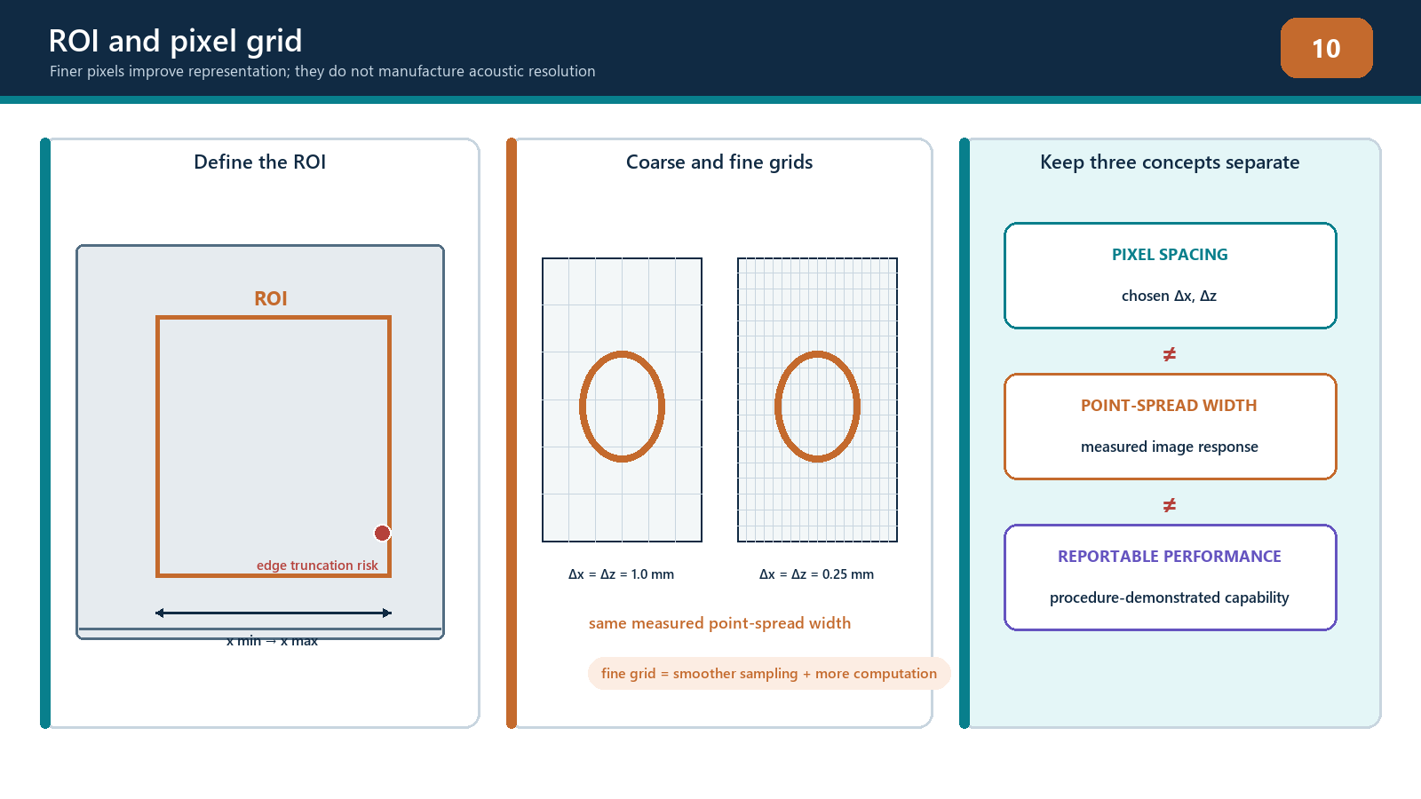
Grid selection should be based on measured amplitude stability or fidelity, location stability, smallest relevant feature separation and practical computation. A wavelength fraction may be a useful starting hypothesis, but there is no universal ratio that proves compliance for every signed-RF, enveloped or proprietary implementation. Verify the final setting on the actual path and target type required by the procedure.
ROI design
The ROI should cover the required examination volume and justified margins without becoming an uncontrolled canvas. Define:
minimum and maximum scan-direction coordinates;
minimum and maximum depth or through-wall coordinates;
the surface/profile reference;
zones assigned to different path views;
overlap between adjacent zones or probe positions;
exclusions such as wedge, air or physically inaccessible regions; and
the relationship to encoded positions.
The pixel count for a rectangular two-dimensional grid is determined by the number of points along each axis.
N_pix = N_x N_z
The exact endpoint convention must be known. If both boundaries are included, the point count is commonly one more than the span divided by spacing after the prescribed rounding. A one-pixel mismatch can shift or truncate a boundary. Do not assume that two software packages interpret ROI width and grid spacing identically.
ROI boundaries deserve practical challenge. Place or scan a reference target just inside, on and just outside each important boundary. Confirm whether the target is displayed, clipped, handed to an overlapping zone or missed. A reflector response has finite width, so cutting the ROI through its peak can alter measured amplitude and apparent size.
Effective aperture and element directivity
Using every matrix pair is not always equivalent to using every pair effectively. For a pixel near the array centre, many elements may have favourable angles. At a far lateral edge or deep location, only part of the physical aperture may fall within useful directivity and transmission angles. Wedge geometry and critical-angle behaviour can restrict the usable aperture further.
Increasing aperture can narrow the main response in one direction, but may also:
include elements with poor sensitivity or large model error;
increase side structure depending on pitch and weighting;
increase sensitivity to surface-profile error;
add noisy or faulty channels; and
slow reconstruction.
Restricting the aperture can improve robustness in one region while broadening the point response and reducing coherent gain. Sub-aperture selection must be documented by element range or rule, not described vaguely as “optimised.”
Apodisation changes the weighting across the aperture. It can reduce sidelobes at the cost of main-response width or sensitivity. The trade should be measured with representative targets rather than accepted from a generic window-function diagram.
Frequency, bandwidth and filtering
The centre frequency and bandwidth originate in the probe, pulser, receiver, material and propagation path. Reconstruction cannot create missing high-frequency content. High frequencies may support a shorter wavelength and finer potential resolution but attenuate and scatter more strongly. Low frequencies penetrate farther but often produce broader responses.
Filters can improve visibility when they remove out-of-band electronic noise. They can also:
change pulse shape and duration;
shift phase or timing if not designed for zero-phase use;
suppress valid low- or high-frequency defect content;
change coherence calculations;
alter apparent tip separation; and
make comparisons invalid when settings differ.
Record the acquisition filter separately from any reconstruction or display filter. Reprocessing a stored full-band dataset with a different filter may be legitimate within a controlled study; silently changing the filter during evaluation is not.
Averaging, smoothing and interpolation
Acquisition averaging can reduce uncorrelated noise when the component and probe remain stationary, but it increases acquisition time and may blur data if the probe moves. Spatial smoothing or image filters can reduce pixel-to-pixel variation, yet they can also merge close reflectors, reduce peaks or fill gaps.
Interpolation can occur in time, image coordinates or display resizing. Each has a different purpose. Time interpolation estimates waveform values at fractional delays. Spatial interpolation resamples the calculated image. Display resizing changes how pixels appear on screen. A smoother display is not evidence of improved acoustic resolution.
The controlled record should state which data are original calculations and which are post-processed presentation. When sizing, use the quantity and processing route authorised by the procedure.
Dynamic range, clipping and normalisation
Receiver clipping occurs before reconstruction when an elementary A-scan exceeds the digitiser range. The clipped waveform has lost amplitude and phase shape. Lowering the final image colour scale cannot restore it. Inspect raw channel peaks, especially front-surface, backwall and large geometry echoes.
Image saturation can also refer to a display maximum. A calculated value above the colour scale may be painted the same colour as a smaller value. This is a presentation limit, but it can hide relative differences.
Normalisation commonly expresses each image relative to its own maximum or a selected reference. Per-image normalisation is useful for seeing weak patterns but dangerous for cross-image comparison: a noisy view and a strong verified view can both show 100%. Record whether scaling is absolute, reference-based, group-based or independently normalised.
Thresholding hides values below a selected level. It can make an image look clean while removing weak tips or splitting a continuous response. Persistence or maximum-hold functions can retain transient peaks after coupling has changed. These controls require declared settings and reset rules.
Coverage versus sensitivity
Coverage has at least three parts:
geometric coverage: a modelled route connects aperture, target region and receiver;
acoustic sensitivity: the complete system produces usable response from representative targets throughout that region; and
encoded coverage: physical scan motion and increment sample the component without unacceptable gaps.
An ROI proves none of these alone. A sensitivity map may show predicted relative response across pixels, but its assumptions about point reflectors, material and surface must be stated. Demonstration blocks should include difficult positions and orientations. If a reference target disappears near an ROI edge, the solution may require another view, probe position or zone—not a brighter colour map.
Computation and data scale
For a straightforward time-domain TFM, work grows with the number of views, pixels, transmitters and receivers.
work proportional to N_views N_pix N_pair
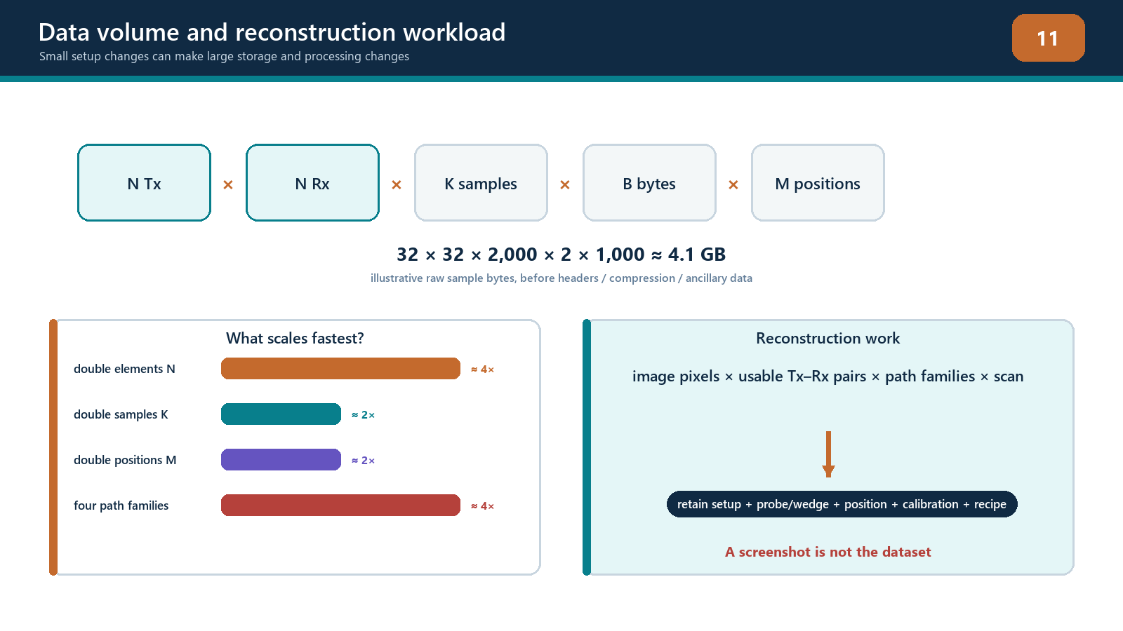
Halving pixel spacing in both axes makes roughly four times as many pixels in a fixed two-dimensional ROI. Adding twice as many views doubles the reconstruction work. Moving from a 32-element square matrix to a 64-element square matrix increases pair count from 1,024 to 4,096 before any pixel increase. Three-dimensional grids add another spatial dimension.
Raw waveform payload also grows with pair count, samples, bit depth and encoded positions. Compression or reduced acquisition may improve practicality, but it can remove the ability to reproduce another reconstruction. Document what is retained and what has been irreversibly discarded.
Frame rate and scan speed are therefore technique variables. If the instrument cannot complete and store each required acquisition at the commanded encoder increment, positions may be skipped or data dropped. The correct response is to reduce scan speed, reduce justified workload or change the authorised plan—not to assume the processor somehow caught up.
Field workflow: freezing reconstruction controls
Define required volume, target sizes/orientations and coordinate tolerance.
Select justified propagation views before optimising display.
Establish a baseline ROI, grid, aperture, filter and scaling.
Check raw data for clipping, noise, channel health and adequate time range.
Change one parameter at a time over a planned range.
Measure peak position, point-spread widths, separability, amplitude stability, background, processing time and data size.
Repeat at central, edge, shallow and deep target positions.
Reject settings that improve one demonstration while failing another required region.
Choose the coarsest grid and smallest workload that still meet all declared performance criteria with margin.
Save the complete setup and version record.
Re-open and reproduce the reference result.
Escalate any unresolved trade-off that affects procedure coverage or acceptance.
Practical 8 — Controlled parameter-sensitivity study
Aim
Reconstruct one FMC dataset through a planned parameter matrix and justify a final controlled setup using measured evidence.
Resources
a verified FMC dataset containing at least two closely spaced targets and targets near ROI boundaries;
access to raw A-scans;
software that permits controlled ROI, grid, aperture, filter and display changes;
timing or processing log;
a fixed measurement worksheet; and
a reference setup protected from accidental overwrite.
Method
Verify dataset identity and create an untouched baseline reconstruction.
Select three grid spacings spanning coarse, expected and fine values.
Translate the ROI origin by part of one coarse pixel while retaining the same physical volume.
Record peak amplitude, peak coordinate and apparent width for each target.
Apply at least three aperture choices: full declared aperture, a justified central sub-aperture and a deliberately excessive restriction.
Apply one documented filter change and one smoothing setting, returning to baseline between changes.
Compare fixed absolute scaling with per-image normalisation.
Measure whether the close targets remain separable under the declared criterion.
Record reconstruction time, frame rate if available, file size and any dropped-data warning.
Repeat key checks for a shallow, deep and lateral-edge target.
Select a final parameter set and state why rejected settings fail.
Save, close, reopen and reproduce the selected setup.
Evidence to retain
parameter matrix with one variable per comparison;
unaltered and reconstructed dataset identifiers;
point-response measurements and coordinates;
amplitude/grid stability results;
processing time and data-volume results;
screenshots using both fixed and normalised scales;
final setup file with checksum or controlled identifier; and
a signed justification linked to the required examination volume.
Stop rules
Stop if the baseline data are clipped or incomplete; settings cannot be changed independently; target identity or true position is unknown; software silently renormalises images; the ROI excludes part of a required response; dropped acquisitions occur; or a fine grid is being selected solely because it displays more decimal places. Do not smooth, threshold or normalise away a failed target.
Common traps
Reporting pixel spacing as physical resolution or sizing accuracy.
Using one central reference target to prove the whole ROI.
Comparing independently normalised images by colour brightness.
Calling display saturation receiver clipping, or overlooking actual clipped A-scans.
Applying smoothing before establishing unsmoothed performance.
Restricting an aperture to remove an artifact without checking lost coverage.
Selecting a universal wavelength fraction without amplitude-stability testing.
Extending the ROI to claim coverage.
Ignoring out-of-plane response in a two-dimensional image.
Freezing settings without recording software and algorithm versions.
Chapter summary
TFM image quality depends on acoustic physics and reconstruction sampling. Axial, lateral, angular and out-of-plane responses differ. Pixel spacing determines where the calculation is sampled; it does not determine the physical point-spread width. ROI boundaries define computation, not coverage.
Effective aperture, directivity, frequency, bandwidth, interpolation, filters, averaging and display controls all change what the operator sees. Clipping destroys source information, while normalisation and thresholds can disguise important differences. Final settings should follow a one-variable-at-a-time sensitivity study across difficult positions and targets. The controlled technique uses measured stability, separation, coverage and processing evidence—not whichever setup produces the smoothest picture.
Study and revision only. This is not an approved inspection procedure, acceptance criterion or qualification.