
CHAPTER 20 · Ultrasonics Level 3
Characterising Probes and the Complete Ultrasonic System
In this chapter · 22 sections
Why this matters
Two probes can carry the same model number and nominal frequency yet produce visibly different A-scans; one may give a short, clean pulse while the other rings, loses sensitivity or sends its strongest energy away from the expected axis. A Level 2 technician can recalibrate both probes and obtain a reference echo. Level 3 must decide whether the probes are interchangeable for the actual technique. That decision requires measured time, frequency, spatial and stability properties linked to detection, location or sizing, rather than faith in a catalogue label.
What you already need
- The practical effects of frequency, bandwidth, pulse length and beam width.
- Reference sensitivity, decibel comparison and signal-to-noise concepts.
- Basic probe, cable, wedge, pulser, receiver and digitiser roles.
- The difference between a probe test and a complete-system check.
- Simple addition of independent variance or uncertainty components.
What you will learn
- Define a task-linked characterisation plan.
- Interpret time, frequency, sensitivity, noise and beam measurements.
- Explain why a beam map is a measurement rather than a photograph.
- Separate probe, channel, coupling and electronic causes of change.
- Distinguish repeatability, reproducibility and stability.
- Make a bounded substitution decision from measured evidence.
Words you will meet
- Characterisation: measurement of properties that influence a stated task.
- Impulse response: time response of a system to a sufficiently short excitation.
- Frequency response: change in amplitude and phase across frequency.
- Bandwidth: stated frequency interval meeting a defined response criterion.
- Transfer function: mathematical description of how one system stage changes a signal.
- Beam map: spatial response measured with a stated target and method.
- Repeatability: variation under closely repeated conditions.
- Reproducibility: variation when relevant conditions such as operator or setup change.
- Stability: behaviour of a measured property over time or environment.
- Comparability: task-linked evidence that two systems support the same claim.
Depth guide for this chapter
- Understand here: what each property means physically and which claim depends on it.
- Calculate here: bandwidth, signal-to-noise, sampled beam width and combined variation.
- Derive later: formal time-to-frequency transformation, system identification and variance models are treated in Chapters 64, 67, 69 and 78.
20.1 The familiar Level 2 comparison
Suppose Probe A and Probe B are both labelled 5 MHz and use wedges with the same nominal angle; on the same reference, Probe A produces a two-cycle pulse and Probe B produces a longer ring-down. Probe B is also 1.5 dB less sensitive and its mapped maximum is displaced laterally. Both can be calibrated to place the reference echo at the correct range.
Calibration corrects selected outputs; it can compensate for a stable delay and can establish a chosen reference sensitivity. It does not make pulse duration, beam axis, bandwidth or stability identical. Those differences matter differently according to the technique. A time-of-flight method may tolerate a modest amplitude difference and still fail if the long pulse merges two arrivals. An amplitude-drop sizing method may be sensitive to beam width. A detection method in coarse material may depend strongly on low-frequency energy and stable signal-to-noise.
The Level 3 starting rule is simple; characterise what the claim depends on. A long list of impressive measurements is not a substitute for that link.
20.2 Define the object being measured
The word probe is often used loosely; a bench test may measure an unequipped transducer on a defined electrical load. A wedge-mounted test includes the wedge and interface. A complete pulse-echo test includes pulser, cable, transducer, wedge, reference target, receiver, digitiser and processing. Results from one boundary do not automatically transfer to another. Construction, damping, electrical loading, wear and repair can cause variation among nominally similar probes; reference-block and probe-characterisation research documents variation and the importance of the complete test arrangement. [R010] A catalogue specification describes design intent. It does not prove the current behaviour of a particular serialised assembly.
A useful characterisation plan names three items before testing:
- The output required by the technique, such as arrival time, peak amplitude or spatial coverage.
- The system boundary included in the test.
- The metric, target, environment and uncertainty used for comparison.
This structure prevents a probe-only result from being reported as complete-system capability; it also prevents an acoustic field difference from being blamed on the receiver before electrical evidence is considered.
20.3 Time and frequency behaviour
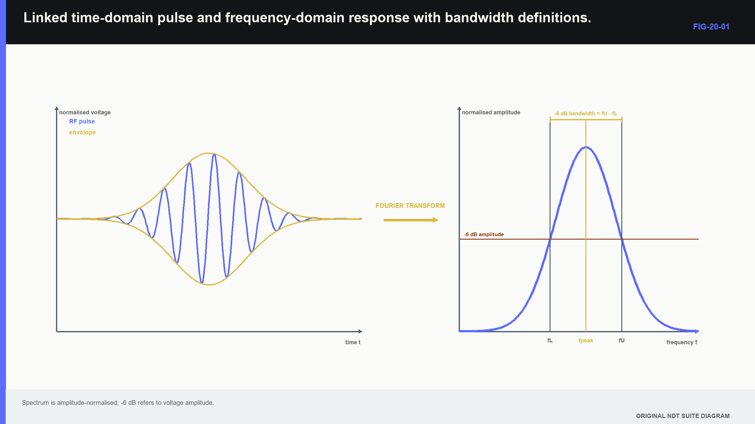
An impulse response is the time-domain output produced by a sufficiently short input within the system bandwidth; a transducer cannot be driven by an ideal infinitely short impulse, so practical tests use a repeatable excitation and reference path. Pulse duration and ring-down affect near-surface recovery and axial separation.
The frequency response describes amplitude and phase change with frequency. A Fourier transform converts a time waveform into a frequency description, and its magnitude supplies the spectral response under suitable conditions. Centre frequency may be defined by spectral peak or by the midpoint between cutoff frequencies. The definition must accompany the number. Bandwidth likewise requires a cutoff convention, such as the two amplitude points 6 dB below the chosen reference.
The figure below connects pulse shape and spectrum; notice that frequency values depend on the declared response and threshold, while pulse duration depends on the declared envelope or crossing rule.
| Worked example · Calculating centre frequency and fractional bandwidth WE-20-01 Given: A probe-system spectrum has -6 dB amplitude points at 3.2 MHz and 6.8 MHz. Centre frequency is defined as their arithmetic midpoint. Find: Centre frequency, absolute bandwidth and fractional bandwidth. Steps: Calculate f_c = (3.2 + 6.8)/2 = 5.0 MHz. Calculate absolute bandwidth, BW = 6.8 - 3.2 = 3.6 MHz. Divide by centre frequency: 3.6/5.0 = 0.72. Answer: Centre frequency is 5.0 MHz, -6 dB bandwidth is 3.6 MHz and fractional bandwidth is 72%. Technical implication: The values describe this measured system, loading and cutoff convention. A different centre definition or electrical load can give a different result. Common mistake: Reporting only “5 MHz” discards the measured bandwidth and the definition that produced the centre value. |
|---|
Time and frequency descriptions are linked; a heavily damped broad-band response is commonly short, while strong resonance creates longer ring-down. That tendency is not an exact one-number conversion for every waveform. The complete pulse shape, spectrum, phase and processing determine the observable result.
20.4 Sensitivity, noise and usable range
Sensitivity is response to a declared target under stated conditions; it has little meaning without noise, stability and saturation. A high response that varies with remounting may be less useful than a lower but stable response. A signal-to-noise value must state whether the signal and noise metrics use peaks, root-mean-square values, image values or band-limited measures. For amplitude-like metrics measured in the same units and bandwidth, the familiar ratio is retained.
| (20.1) Signal-to-noise ratio in amplitude decibels · EQ-20-02 Where: SNR_dB = signal-to-noise ratio (dB); A_signal = declared signal metric; A_noise = noise metric in the same units and bandwidth Model limits: comparable amplitude-like metrics and stated measurement windows |
|---|
The observable is a declared signal-to-noise comparison, not a universal property of the reflector; changing the noise window, filter or metric can change the result. The relationship supports comparison only when those choices remain consistent. Linearity establishes whether amplitude changes are represented proportionally across a range; reserve gain or headroom protects against clipping when unexpected large responses occur. Recovery time controls whether a weak signal can be observed after a strong pulse or interface echo. Temperature cycling, cable movement and remounting can reveal instability that a single bench reading misses.
| Worked example · Separating sensitivity drift from reference variation WE-20-02 Given: A daily acoustic reference response falls 2.5 dB. A second independent acoustic reference falls 2.4 dB, while an electrical receiver self-test is unchanged. Re-coupling restores both acoustic responses. Find: The leading cause category. Steps: Compare the evidence layers. Two acoustic paths change together. The electrical receive reference does not change. Re-establishing the acoustic interface restores both responses. Answer: Coupling or the common acoustic interface is the leading cause, rather than receiver gain. Technical implication: Independent reference layers localise the change and prevent unnecessary adjustment of stable electronics. Common mistake: Adjusting gain immediately destroys the original signature and can hide an unstable interface. |
|---|
20.5 Beam maps are measured responses
A beam map is sometimes treated as a photograph of sound; it is actually the response of a field interacting with a mapping target, sampled by a positioning system and processed by an amplitude or energy metric. The target is therefore part of the measurement. A small ball or wire can sample a local region but may give a weak and directional response; a long side-drilled hole integrates the field along its length. A hydrophone measures pressure in water and can average over its active area. A solid pulse-echo target includes transmission, scattering and reception. These methods answer related but not identical questions.
Useful outputs include axis position, focal position, -6 dB width, side-lobe level, skew and change with depth; the map applies to the mode, frequency band, medium, target and setup used. Transfer into another component requires a physical argument and confirming evidence. Spatial step limits the map; a grid as wide as the expected beam can miss the true maximum and distort the apparent width. A finer grid cannot undo averaging by a large target. Position accuracy, target location, alignment, temperature and interpolation all contribute to uncertainty.
Measured low-frequency fields in coarse cast stainless systems illustrate why an ideal source model alone can be inadequate when material structure distorts the propagated field. [R011] [R012]
| Worked example · Quantifying beam-width uncertainty from a sampled map WE-20-03 Given: A lateral map is sampled every 0.50 mm. Linear interpolation places the -6 dB crossings at -3.25 mm and +3.55 mm. Position repeatability contributes 0.15 mm standard uncertainty to each crossing, and amplitude with interpolation contributes an equivalent 0.20 mm. Treat the two crossings as independent. Find: Beam width and its standard uncertainty under this model. Steps: Width is 3.55 - (-3.25) = 6.80 mm. Each crossing has uncertainty sqrt(0.15^2 + 0.20^2) = 0.25 mm. Combine the independent crossing uncertainties: sqrt(0.25^2 + 0.25^2) = 0.35 mm. Answer: Mapped -6 dB width is approximately 6.80 +/- 0.35 mm standard uncertainty. Technical implication: The map supports a width with a meaningful resolution. It does not support three decimal places or an unqualified transfer to another target and medium. Common mistake: Treating interpolated crossing coordinates as exact confuses numerical display precision with spatial knowledge. |
|---|
Repeat maps separate persistent structure from setup variation; a side lobe that returns at the same coordinate is likely a stable field feature. A wandering maximum may indicate alignment, coupling or reference error. Difference maps can reveal wedge wear or element loss before a single peak-amplitude check crosses a limit.
20.6 The complete-system response
In approximately linear operation, each stage modifies the signal; excitation has a spectrum. The transmitter converts it into a field. Propagation changes amplitude and phase. The target scatters the incident field. Reception and digitisation add their own response. Processing then creates the stored or displayed representation. The frequency-domain product is a compact map of these dependencies.
| (20.2) Pulse-echo system spectrum · EQ-20-01 Where: Y = measured spectrum; E = excitation spectrum; H_T = transmit conversion and field response; H_P = propagation response for outward and return paths; H_S = scatterer response; H_R = receive transducer and analogue response; H_D = digitiser and processing response Model limits: approximately linear time-invariant behaviour over the observation and no unrepresented mode coupling |
|---|
This equation explains why measured centre frequency is a system property; a broad transducer driven through a narrow receiver produces a narrow measured band. A cable resonance or digital filter can reshape a pulse attributed incorrectly to the probe. Pulse-echo response involves transmit and receive conversion, but it should not automatically be described as a simple square because loading, target and propagation remain. The product supports dependency reasoning and comparative tests; separating every factor by deconvolution requires adequate signal-to-noise, reference knowledge and model control. Noise can be amplified. Nonlinearity also breaks the simple transfer description. Pulser saturation, receiver clipping, automatic gain, thresholding and envelope compression make the output depend on level or signal history.
At Level 3, the learner should interpret a supplied transfer response and identify likely confounding stages; Fourier derivation, convolution, deconvolution and system identification are developed in Chapter 64.4 and Chapters 69.1, 69.12 and 69.15.
20.7 Element and channel condition
Array systems add per-element excitation, sensitivity, noise, timing and cross-talk; a complete aperture can pass an overall sensitivity check while containing weak, noisy or mistimed elements. Coherent addition makes phase and timing important as well as amplitude. The field consequence depends on location; losing an edge element narrows active aperture and can broaden the main lobe. Losing a central element can raise side-lobe structure. A contiguous group can create an asymmetric field and shift its centroid. A rule allowing a number of dead elements without considering position, aperture and task is physically incomplete.
Diagnosis should separate element conversion, electrical channel, cable path and acoustic coupling; channel substitution, electrical reference loads and transmit-receive comparisons can divide the hypotheses when supported by the equipment. A channel map should retain individual metrics, not only a pass count. Dual-element conventional probes have a related issue; transmit and receive imbalance changes the overlap region. Angle-probe wedge wear changes delay, index and angle. A complete-system baseline allows those patterns to be compared before degradation becomes obvious on production data.
Studies of low-frequency arrays in coarse cast stainless systems demonstrate why measured apertures and actual material propagation matter when ideal fields are distorted. [R011] [R012] The general lesson is that element condition must be linked to field and task, not reduced to a hardware tally.
20.8 Repeatability, reproducibility and stability
Repeatability describes closely repeated conditions, such as repeated readings without changing the operator, fixture or day. Reproducibility includes deliberate changes expected in use, such as remounting, operators, probes or days. A stable instrument can coexist with poor reproducibility when placement and coupling dominate. Stability adds time; immediate repeats do not reveal warm-up drift, daily setup variation, temperature coefficients, cable intermittency, wedge wear or ageing. The monitoring period should match the period over which the baseline supports decisions.
Control data can include delay, reference amplitude, noise, centre frequency, bandwidth, beam-axis position and channel metrics; statistical limits describe unusual change relative to a stable baseline. Engineering limits describe change large enough to matter to the claim. The two are not the same. A statistically unusual 0.1 dB shift may be irrelevant to a time-of-flight result, while a 1 mm index change may matter even if similar variation occurred historically.
Environmental and mechanical challenges help identify mechanisms; temperature cycling estimates reversible coefficients. Flexing a cable while monitoring noise reveals intermittency. Remounting estimates registration contribution. These tests explain variation instead of merely collecting repeated numbers.
20.9 Technical decision case: where improvement has leverage
| Worked example · Interpreting a simple reproducibility budget WE-20-04 Given: Estimated standard-deviation components for measured beam index are repeatability 0.20 mm, remounting 0.45 mm, operator 0.25 mm and day-to-day environment 0.15 mm. Treat the components as independent for this example. Find: Combined reproducibility standard deviation and the dominant contribution. Steps: Combine variances: s_R = sqrt(0.20^2 + 0.45^2 + 0.25^2 + 0.15^2). The sum of variances is 0.3275 mm^2, giving s_R = 0.572 mm. Remounting contributes 0.45^2/0.3275, about 62% of total variance. Answer: Combined reproducibility standard deviation is about 0.57 mm, with remounting the dominant component. Technical implication: Better fixture registration offers greater improvement than extra digitiser resolution. The physical budget directs effort to the dominant source. Common mistake: Adding standard deviations directly produces an unnecessarily large value and ignores the stated independent-variance model. |
|---|
This calculation is suitable when components and independence are supplied; a full crossed study may include probes, operators, days, repeats and interactions. Interactions matter because one operator may work particularly well with one fixture, or one probe may be unusually temperature-sensitive. Chapter 78.5 and Chapter 78.12 develop designed measurement-system studies and variance-component models.
20.10 A task-linked substitution decision
Substitution begins with the output; a time-of-flight location technique may prioritise delay stability, beam axis, adequate timing bandwidth and signal-to-noise. An amplitude-drop sizing technique places greater weight on beam profile, pulse shape, sensitivity linearity and coupling stability. An array method also depends on element condition, phase, steering response and compatibility with the declared laws. Three conclusions are possible; equivalent task-linked outputs within justified tolerances support substitution. A stable correctable difference, such as constant delay, can support substitution after correction and targeted comparison. A changed field, resolution or target response can require technique revision or renewed demonstration.
Return to the opening probes; if Probe B has longer ring-down and a displaced beam axis, a simple gain and zero calibration does not establish equivalence. Time-of-flight use may survive after timing and axis evidence show adequate performance. Close-tip sizing or beam-based amplitude sizing may require a new demonstration. The conclusion depends on the claim, not the desire to approve or reject the hardware. A technical fingerprint combines time response, spectrum, sensitivity, noise, field, repeatability and stability with uncertainty; mean agreement alone is insufficient if one system has much greater remount variability. A retained fingerprint also supports later diagnosis after damage or repair by showing whether change is delay, gain, spectral loss, axis movement or noise.
20.11 Formal depth and the Part VIII handoff
The Level 3 learner is expected to design characterisation, calculate common metrics and make a task-linked comparison. Full derivation and device engineering continue later:
- Chapter 64.4 develops Fourier transforms, convolution and correlation.
- Chapter 64.8 develops covariance and dependence.
- Chapter 67 treats piezoelectric coupling, backing, matching, cross-talk and tolerances.
- Chapter 69 treats system response, estimation and processing-chain validation.
- Chapter 78 treats uncertainty, designed experiments and reproducibility.
Those chapters explain how the models are built; this chapter establishes which physical measurement each model must support.
In plain words
- Nominal model and frequency labels do not prove interchangeability.
- Characterisation should measure properties on which the technique claim depends.
- Pulse duration, bandwidth, sensitivity, noise and beam shape answer different performance questions.
- A beam map includes the mapping target, positioning and processing method.
- Complete-system response can differ from isolated transducer response.
- Weak or mistimed elements change an array field according to their position.
- Repeatability, reproducibility and stability describe different kinds of variation.
- Substitution is supported by task-linked output evidence and uncertainty.
Key terms
- Characterisation: measurement of task-relevant system properties.
- Impulse response: time response to a sufficiently short excitation.
- Bandwidth: declared frequency range meeting a response criterion.
- Transfer function: stage-by-stage signal modification model.
- Beam map: target- and method-dependent spatial response measurement.
- Repeatability: variation under closely repeated conditions.
- Reproducibility: variation after relevant conditions change.
- Stability: behaviour over time or environment.
- Comparability: evidence that systems support the same task-linked output.
Key relationships
- fractional bandwidth = (f_high - f_low)/f_c: bandwidth requires declared cutoff and centre definitions.
- SNR_dB = 20 log10(A_signal/A_noise): signal and noise metrics must be comparable.
- Y = E H_T H_P H_S H_R H_D: measured spectrum reflects the complete linearised chain.
- s_R = sqrt(sum of component variances): independent standard-deviation components combine through variance.
Common mix-ups
- Calibration is not complete characterisation.
- A beam map is not a target-free photograph of pressure in the component.
- Sample count of failed elements does not describe their field consequence.
- Statistical control limits are not automatically engineering acceptance limits.
- Catalogue identity is not measured complete-system equivalence.
Bridge to Chapter 21
Chapter 20 treated the instrument as one stage inside the assembled system; chapter 21 isolates instrument and digital-data behaviour. It starts with visible errors such as flattening, drift and dropped records, then connects them to timing, amplitude, filtering and acquisition integrity.
Sources and further study
- [R010]
- [R011]
- [R012]
Study and revision only. This is not an approved inspection procedure, acceptance criterion or qualification.