
CHAPTER 47 · FMC / TFM / PCI Level 2
Reading the Transmit-Receive Matrix
In this chapter · 22 sections
Why this matters
One FMC position can contain thousands of A-scans; the volume looks complicated until the learner gives every trace an address. A row names the transmitter, a column names the receiver, and the cell between them contains one familiar waveform. That simple grid reveals missing transmit events, weak receiver channels and pair-specific faults before a reconstruction hides them inside a smooth image. It also provides the bridge into phase: the waveform sign and cycle position must be preserved when later processing depends on coherent alignment.
What you already need
- The Chapter 46 distinction between FMC acquisition and TFM reconstruction.
- The PAUT meaning of an element number and a stored A-scan.
- Basic time-base, sample-rate, coupling, noise and clipping awareness.
- The idea that a pulse contains repeating positive and negative radio-frequency (RF) cycles.
- Confidence using multiplication and simple fractions.
What you will learn
- Locate any transmitter-receiver A-scan in a matrix.
- Use diagonal, row and column patterns to form fault hypotheses.
- Calculate ordered and reciprocal pair counts without assuming equivalence.
- Explain phase as position within a repeating waveform.
- Estimate how a timing offset changes phase.
- Identify the metadata needed before a matrix can be reconstructed responsibly.
Words you will meet
- Matrix cell: one A-scan identified by its transmitter row and receiver column.
- Diagonal: the cells in which the transmitting and receiving element numbers match.
- Off-diagonal: cells in which different elements transmit and receive.
- Radio-frequency waveform: the signed, oscillating signal stored before envelope display.
- Phase: position within a repeating cycle.
- Reciprocity: the expectation that reversed acoustic transfer can be comparable under stated conditions.
- Metadata: information that explains the identity, timing, geometry and processing context of data.
47.1 Picture the matrix as a labelled board
Imagine a square board; the numbers down its left edge identify transmitting elements. The numbers across its top identify receiving elements. Choose row 3 and column 11; the cell at their crossing contains the A-scan recorded when element 3 transmitted and element 11 received. This book calls that ordered trace A_3,11, or more generally A_ij for transmitter i and receiver j.
Move across one row and the transmitter stays fixed while the receiver changes. Move down one column and the receiver stays fixed while the transmitter changes; the matrix therefore does more than store traces. Its shape connects signal behaviour to the job performed by each channel.
The main diagonal contains cells such as A_1,1, A_2,2 and A_3,3. Each uses the same physical element for transmit and receive at different times in the electronics, so the geometry resembles pulse-echo. An off-diagonal cell such as A_3,11 uses a pitch-catch path; its total route runs from element 3 to the interaction and then from the interaction to element 11.
The next figure makes one cell visible inside the larger grid. Notice that the cell contains a complete A-scan over time, not one amplitude number.
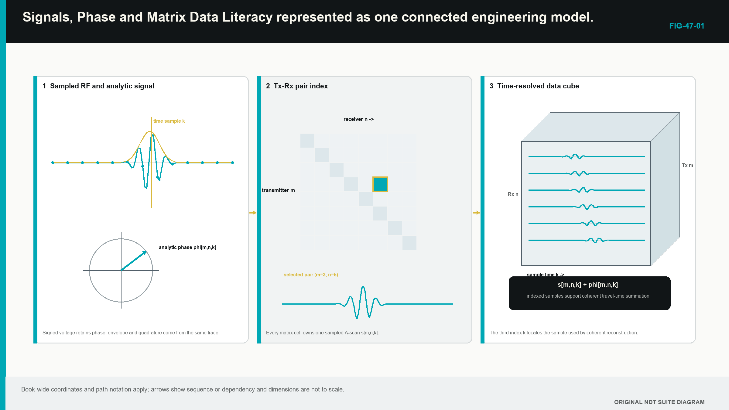
This board picture should be stable before thinking about TFM. Reconstruction later visits different times in different cells; it does not change what the cells contain.
47.2 Read rows, columns and isolated cells
A weak row means that one transmit event produced weak data across many receivers. The cause may be the physical element, the pulser selection, the transmit connection, unstable contact during that firing or a sequence error. A weak column means that one receiver was weak across many transmit events; that pattern points first toward a receiver path, channel assignment or physical element response in reception.
When the same element number has a weak row and weak column, a shared physical cause becomes more credible. The element, connector, wiring or local coupling under that part of the aperture may be involved. One isolated bad cell suggests a trace-specific acquisition, transfer or file problem rather than complete loss of the element.
Patterns guide a test; they do not prove a component has failed. Transmit and receive electronics perform different jobs. One physical element can behave differently in those roles. A multiplexed system can also map logical channels to physical elements in a way that is not obvious from the display. The technician confirms the element map, repeats the reference acquisition and uses the approved channel check before excluding data or replacing hardware.
The final TFM image can disguise these patterns. Thousands of healthy contributions may make one failed row look harmless. Matrix health should therefore be checked at the data level, not inferred solely from image smoothness.
47.3 Count ordered pair traces
One full row contains one trace for every selected receiver. Repeating the row for each transmitter gives the ordered trace count. The relationship is the same physical count introduced in Chapter 46, now tied directly to the board.
| (47.1) Ordered FMC trace count · EQ-47-01 Where: N_trace = ordered transmitter-receiver traces at one position (count); N_tx = selected transmit events (count); N_rx = separately recorded receivers per event (count) Model limits: every declared ordered transmitter-receiver combination is acquired and retained once |
|---|
A 32-transmitter by 48-receiver record contains 32 x 48 = 1,536 traces per position. That count is not a square full matrix because the transmit and receive populations differ, but it is still a clearly defined ordered matrix.
For a square matrix, some techniques use acoustic reciprocity to justify retaining only one member of each reversed pair. If the diagonal is included, the arithmetic count of unique unordered pairs is:
| (47.2) Unique unordered pair count with diagonal · EQ-47-02 Where: N_unique = unordered element pairs including self-pairs (count); N = common selected transmit and receive element count (count) Model limits: a square matrix and a separately demonstrated basis for treating reversed pairs as equivalent for the intended use |
|---|
For 64 elements, N_unique = 64 x 65 / 2 = 2,080 pairs. The full ordered count remains 4,096. The smaller number describes a possible reduced record; it does not rewrite the acquisition history. A technique using the reduction must show that the missing order does not remove information required for its paths, diagnostics or performance.
47.4 Reciprocity is a comparison, not a promise
Reverse one off-diagonal pair. A_3,11 and A_11,3 exchange transmitter and receiver. In a stable, linear and reciprocal acoustic system, important transfer features can be similar. Arrival timing, pulse form and usable frequency content can therefore provide a useful consistency comparison.
Exact sample equality is not expected. The first event drives element 3 with a pulser and listens through the receiver connected to element 11. The reverse event occurs later in the sequence with the electronic roles exchanged. Coupling can change between firings, transmit and receive bandwidths can differ, and the two records may use different gains or channel corrections.
A large unexplained difference is a diagnostic lead. Timing disagreement can point to channel delay or trace assignment. Frequency-shape disagreement can point to electronics, wiring or contact. A difference that changes along the encoded scan can point to motion or coupling. Clipping can affect one direction more strongly because the drive and return conditions differ.
Open FMC sources describe the matrix as ordered pair data and emphasise timing, trace identity and phase-preserving acquisition for coherent reconstruction. They also support using reciprocal structure as evidence that must be checked, not assumed. [R017] [R026]
47.5 Open the A-scan inside a cell
The cell waveform normally begins with a baseline or pre-trigger region. Electrical breakthrough, the initial pulse, wedge activity and the entry surface may follow. Later packets can arise from targets, component boundaries, conversions or reverberations. The useful time window depends on the pair separation and the selected acoustic path.
A diagonal pulse-echo response from a known target may arrive sooner than the corresponding wide off-diagonal response because the pitch-catch route is longer. An electronic event fixed at the same sample across most rows and columns behaves differently. It follows instrument time rather than component path length and can reconstruct as a structured artefact.
View the source waveform as signed radio-frequency (RF) data when phase or coherent addition matters. An envelope makes signal magnitude easier to see, but it removes visible polarity. Rectification can hide asymmetric clipping. A trace normalised to its own maximum hides absolute weakness. If the stored representation has already discarded sign or amplitude, the limitation belongs in the data record.
The useful cell check is modest. Confirm that the required time range exists, the signal is not clipped, the baseline is plausible, relevant packets sit above noise and the trace identity matches the declared pair. It is not necessary to interpret every wiggle as a reflector.
47.6 Phase starts with a clock-face picture
Phase means position within one repeating cycle. Picture a clock face attached to a sine wave. The right-hand crossing can represent 0 degrees. The positive peak is near 90 degrees, the next crossing near 180 degrees, the negative peak near 270 degrees, and the next right-hand crossing begins another cycle.
The circular nature matters. Angles of 359 degrees and 1 degree are close together even though ordinary subtraction appears large. A positive RF sample gives a rough indication of which half-cycle is present, but it does not give the precise phase angle. A sign-only method therefore keeps less phase detail than a full phase representation.
Time and phase are connected. One full period corresponds to 360 degrees. A delay equal to one quarter of the period shifts a single-frequency component by 90 degrees. Higher frequency has a shorter period, so the same timing error consumes a larger part of the cycle.
Real ultrasonic pulses contain a band rather than one endless sine wave. Filtering and bandwidth affect cycle shape. Phase also becomes unreliable where the waveform magnitude approaches noise. Chapter 52 returns to these limits when coherence is used to make an image.
47.7 Turn a timing offset into phase rotation
The practical relationship is stated before its use. Phase rotation equals 360 degrees multiplied by the timing offset divided by the period of the frequency component being considered. This is a comparison scale, not a complete model of a broadband pulse.
| Worked example · Timing error as a phase rotation WE-47-01 Given: A 5 MHz waveform component is sampled at 20 MHz. One channel has a 20 ns timing offset. Find: The samples per cycle and the approximate phase rotation of that component. Steps: A 5 MHz period is 1/5 MHz = 0.20 microseconds = 200 ns. A 20 MHz sampling interval is 1/20 MHz = 50 ns, giving 200/50 = 4 samples per cycle. The phase rotation is 360 degrees x 20 ns / 200 ns = 36 degrees. Answer: The component spans four stored samples per cycle, and the 20 ns offset represents about 36 degrees of phase. What it means in practice: A small channel delay can weaken coherent addition even when the envelope peak still looks close to the expected time. Common mistake: Treating four samples per cycle as proof of adequate signal fidelity ignores analogue bandwidth, filter behaviour and interpolation. |
|---|
The sense-check is direct. Half a period would be 100 ns and 180 degrees. The calculated 20 ns shift is one fifth of that time and one fifth of 180 degrees, giving 36 degrees.
47.8 From a board to a data block
The board has transmitter and receiver axes. Every cell also extends through time samples, so one physical scan position contains a transmitter-by-receiver-by-time block. An encoded scan adds physical position as another dimension.
Two simple slices help the learner navigate it. A fixed-pair view opens one cell through time and looks like an A-scan. A fixed-time view shows the signed value of every pair at one sample. A row-energy view summarises each transmit event. A column-energy view summarises each receiver. These summaries can reveal structure, but they do not replace inspection of representative waveforms.
A TFM pixel samples this block along a model-defined set of times. Each pair has a different predicted arrival, so the contributing values do not come from one flat time slice. Changing velocity or geometry leaves the stored block unchanged while moving the set of times visited by the reconstruction. That is why a feature can sharpen, move or disappear during reprocessing without any new acquisition.
The matrix-data and phase literature also makes an important reliability point. Phase should be interpreted only where signal support is adequate, and the physical pair mapping, time origin, sample rate, filters and channel condition must remain known. [R017] [R026]
47.9 Read common health signatures
A dead or weak physical element can reduce its transmit row, its receive column or both. A receiver-chain fault tends to follow one column across many transmitters. A transmit-sequence fault tends to follow one row. A trace transfer problem can affect an isolated cell or a block of cells. The first action is to preserve the pattern and compare it with a stable reference, not copy a neighbouring trace into the gap.
Saturation has its own signature. Positive or negative peaks flatten at a repeated limit and waveform shape is lost. Strong diagonal or near-surface traces may clip while long paths remain weak, so an image-wide maximum does not prove the complete matrix stayed linear.
Cross-talk and fixed-time interference can occur at similar sample locations across many pairs. After reconstruction, such an event may form a line, arc or repeated hot region. A coupling change tends to follow physical position and can affect several elements together. A position dropout affects an entire matrix or group of matrices at a missing, repeated or wrong coordinate.
A controlled audit therefore checks diagonal, near off-diagonal and wide off-diagonal traces; row and column summaries; selected reciprocal pairs; matrix dimensions; and encoded-position continuity. Any pair exclusions remain visible because they change the effective aperture.
47.10 Metadata gives every number a meaning
Preserve instrument, software and firmware identity; probe, wedge and element map; transmitter and receiver selections; firing order; pulser, gain and filter settings; sample rate, count and time origin; stored signal type; component and velocity model; coordinate origin and array orientation; encoder direction and increment; coupling notes; and the reconstruction recipe used for derived images.
The word raw needs care. An export may already be filtered, rectified, compressed, reduced or converted through proprietary software. The record should state what occurred and which information no longer exists. A large numeric array without pair mapping and timing context is not a reusable FMC dataset. It is an impressively heavy mystery file.
Before reconstruction, the technician confirms that the declared dimensions match the file, representative traces are linear and supported, position links are complete, and required metadata can reproduce the time and geometry model. A fault is then accepted, excluded, reacquired or escalated according to the controlled technique.
47.11 Formal phase signpost
Some processing creates an analytic signal by pairing the real RF waveform with a calculated quarter-cycle-related component. The two components define a magnitude and an angle. At Level 2, the learner uses that picture and does not derive the transform.
The source equation is retained here as a labelled signpost because later PCI and engineering chapters refer to it:
| (47.3) Analytic signal · EQ-47-03 Where: z(t) = complex analytic signal (same signal units as x); x(t) = real RF signal at time t (voltage or digitiser units); t = time (s); H{x(t)} = Hilbert-transform quadrature component (same signal units); j = square root of minus one (dimensionless) Model limits: a linear sampled signal and a declared discrete Hilbert-transform implementation |
|---|
This equation says that processing combines the observed waveform with a related component to form a two-coordinate representation. It is not a Level 2 calculation requirement. Chapters 58 and 59 develop processing order and coherence families at Level 3. Chapters 64.4 and 69.16 derive the transform and phase-estimation tools.
Step up
Chapter 55 compares full, half, sparse and plane-wave acquisition architectures. Chapter 58 treats fractional delay, analytic-signal order and numerical implementation. Chapter 62 develops dataset forensics when row, column, timing or file evidence is abnormal. Those chapters turn the literacy established here into design and diagnostic control. [R017] [R026]
In plain words
- A matrix row identifies one transmitter and a column identifies one receiver.
- Every cell contains one time waveform, not one finished image value.
- Diagonal cells use the same numbered element for transmit and receive; off-diagonal cells are pitch-catch pairs.
- Row and column patterns suggest transmit- and receive-side faults but still need confirmation.
- Reversing a pair gives a useful reciprocity comparison, not guaranteed identical samples.
- Phase is position within a repeating cycle and becomes sensitive to small timing errors.
- TFM visits a different predicted time in each cell when calculating one pixel.
- Metadata connects the stored numbers to real elements, time and component position.
Key terms
- Matrix cell: one ordered transmitter-receiver A-scan.
- Diagonal: cells with matching transmitter and receiver element numbers.
- Off-diagonal: cells with different transmitter and receiver numbers.
- RF waveform: signed oscillatory source signal retained through time.
- Phase: cycle position, expressed as an angle or equivalent fraction of a period.
- Reciprocity: conditional comparison between reversed transfer paths.
- Metadata: identity and context required to understand and reuse data.
Key relationships
- N_trace = N_tx N_rx: ordered trace count follows the complete row-by-column population.
- N_unique = N(N + 1)/2: arithmetic count for one member of each reciprocal pair plus the diagonal, when the reduction is separately justified.
- phase rotation = 360 degrees x delay/period: a timing error consumes a fraction of a cycle.
- matrix + time + position: an encoded FMC record extends the transmitter-receiver board through waveform samples and scan location.
Common mix-ups
- A weak row suggests a transmit-side problem; it does not prove the physical element alone is faulty.
- Reciprocal similarity does not authorise deleting half the matrix.
- Envelope magnitude does not retain the visible RF sign or full phase.
- A high sample rate does not restore analogue bandwidth that was never acquired.
- A TFM pixel does not copy one cell or one fixed-time slice.
Bridge to Chapter 48
Chapter 47 made the matrix readable. Chapter 48 follows the matrix while it is being acquired. It separates problems that remain adjustable in later reconstruction from clipping, missing time, coupling loss and position faults that permanently damage the evidence.
Sources and further study
- [R017]
- [R026]
Study and revision only. This is not an approved inspection procedure, acceptance criterion or qualification.