
CHAPTER 9 · FMC / TFM / PCI Level 2
Phase Coherence Without the Mystique
In this chapter · 16 sections
Purpose
Phase-coherence imaging is easier to understand when phase is treated as a familiar property of the RF waveform rather than a mysterious new measurement. A pulse has cycles. After correct travel-time alignment, samples from a common event can arrive at similar positions within those cycles. Their phase directions agree. Samples caused by unrelated noise often point in different directions. A coherence calculation describes that agreement.
Agreement is useful, but it is not identity. Geometry echoes can be coherent. A valid planar reflector can return energy to only part of the aperture. A weak signal buried in noise has unreliable phase. This chapter develops enough phase literacy to use coherence as evidence without mistaking a high score for proof of a defect.
Learning outcomes
After completing this chapter, the learner will be able to:
distinguish instantaneous phase, polarity/sign and envelope amplitude;
explain why a correctly delayed point-like event can align across channels;
use a generic bounded vector-coherence equation as a conceptual model;
compare coherent signal, coherent noise and phase-inconsistent valid response;
predict how timing, velocity, geometry, filtering and low signal level affect phase agreement; and
state why coherence cannot independently classify or accept a discontinuity.
Crossover map: from RF polarity to phase agreement
| Existing UT/PAUT concept | Coherence crossover |
|---|---|
| The RF trace alternates positive and negative around zero. | Polarity is a coarse phase indicator; full instantaneous phase represents position around the cycle. |
| Delay laws align waveforms for constructive interference. | Pixel-specific delays should align a common event across selected FMC pairs before coherence is assessed. |
| Envelope amplitude removes visible RF sign. | Phase requires the underlying oscillatory or analytic representation; an envelope alone does not contain full phase. |
| Noise can be random or repeatable. | Random phase tends to reduce coherence, but repeatable cross-talk or geometry can remain highly coherent. |
| Wrong velocity shifts an echo position. | It also leaves residual phase differences across channels and can reduce a coherence response. |
| Signal-to-noise ratio matters. | When signal amplitude approaches noise, estimated phase becomes unstable even in an amplitude-free display. |
Phase is circular
One ultrasonic cycle can be described from 0° through 360°, or from −180° through +180°. The end of the interval joins the beginning: 359° and 1° are only 2° apart, not 358°. This circular property matters when calculating phase spread. An ordinary arithmetic average can put two nearly aligned phases on opposite sides of the circle at 180°, which is plainly wrong.
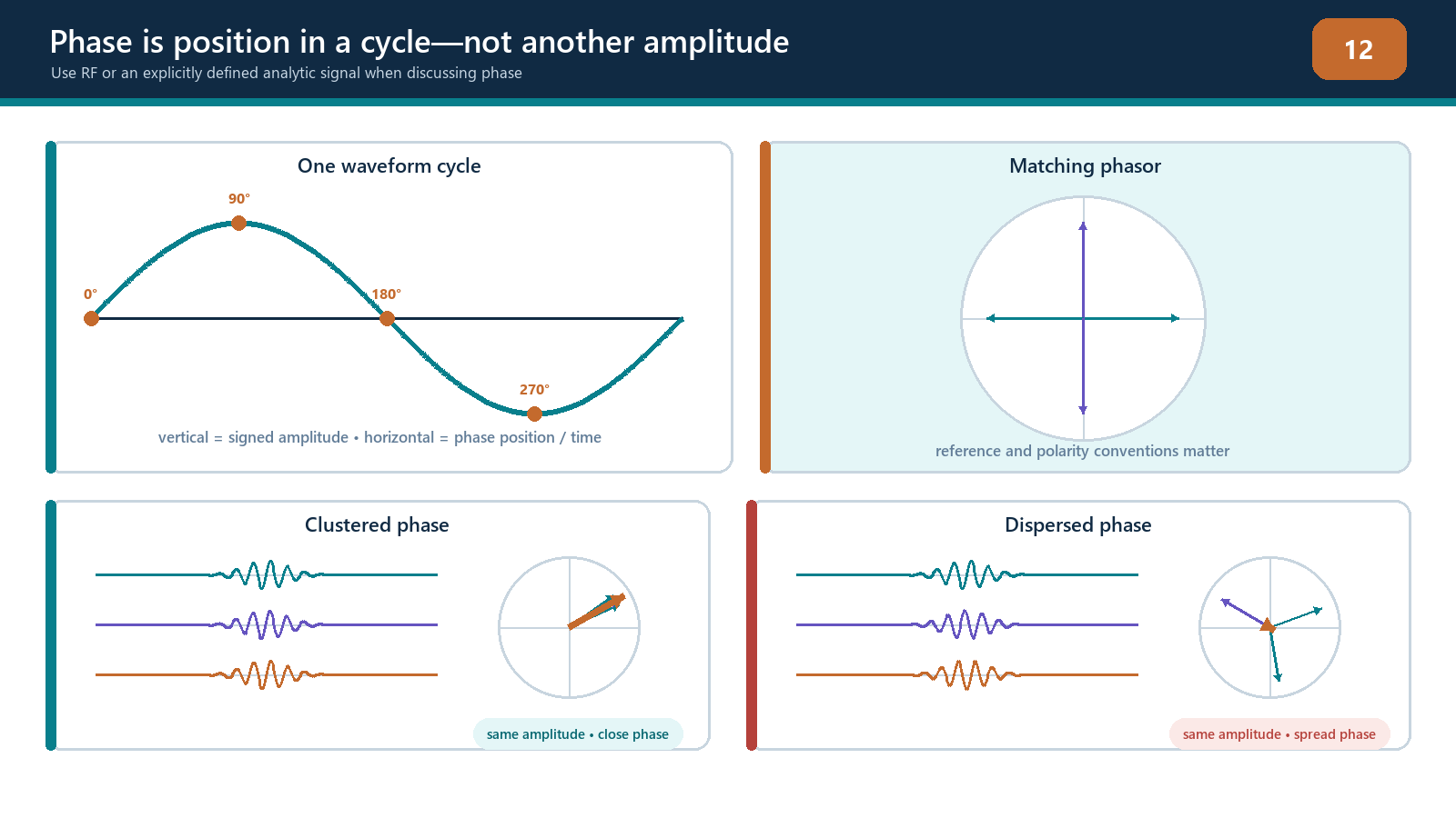
Phase is not the same as time, although a time shift changes phase. For a single frequency f, a delay Δt produces a phase change proportional to f × Δt. A small timing error is therefore a larger fraction of a cycle at high frequency. Real ultrasonic pulses contain a band of frequencies, so their phase behaviour also depends on bandwidth, filtering and the method used to define instantaneous phase.
Polarity is simpler than phase. A positive RF sample can be assigned +1 and a negative sample −1. This indicates which half-cycle the sample occupies but discards its exact angle and amplitude. Sign-coherence methods use this efficient reduction, but they are not identical to full phase-dispersion or vector-coherence methods.
Analytic signal at an applied level
An RF A-scan is a real-valued oscillating signal. Processing can create a quadrature component that is shifted by a quarter cycle relative to it. The original component and quadrature component form an analytic signal. At each time:
the distance from the origin represents envelope magnitude; and
the angle around the origin represents instantaneous phase.
The technician does not need to derive the Hilbert transform to understand the evidence. The important controls are the source RF data, bandwidth, time delay and phase extraction method. If only a displayed envelope is exported, the original phase may no longer be recoverable. If a commercial implementation binarises or retains only signs, it may also discard amplitude irreversibly.
Phasors and alignment
A phasor is an arrow representing phase angle. Imagine one delayed sample from each contributing transmitter–receiver pair:
if the arrows point in nearly the same direction, their vector average remains long;
if they point in many directions, they cancel and the average becomes short;
if half point one way and half point opposite, the vector average can approach zero; and
if only a few reliable arrows exist among many noise arrows, the result depends strongly on aperture and threshold rules.
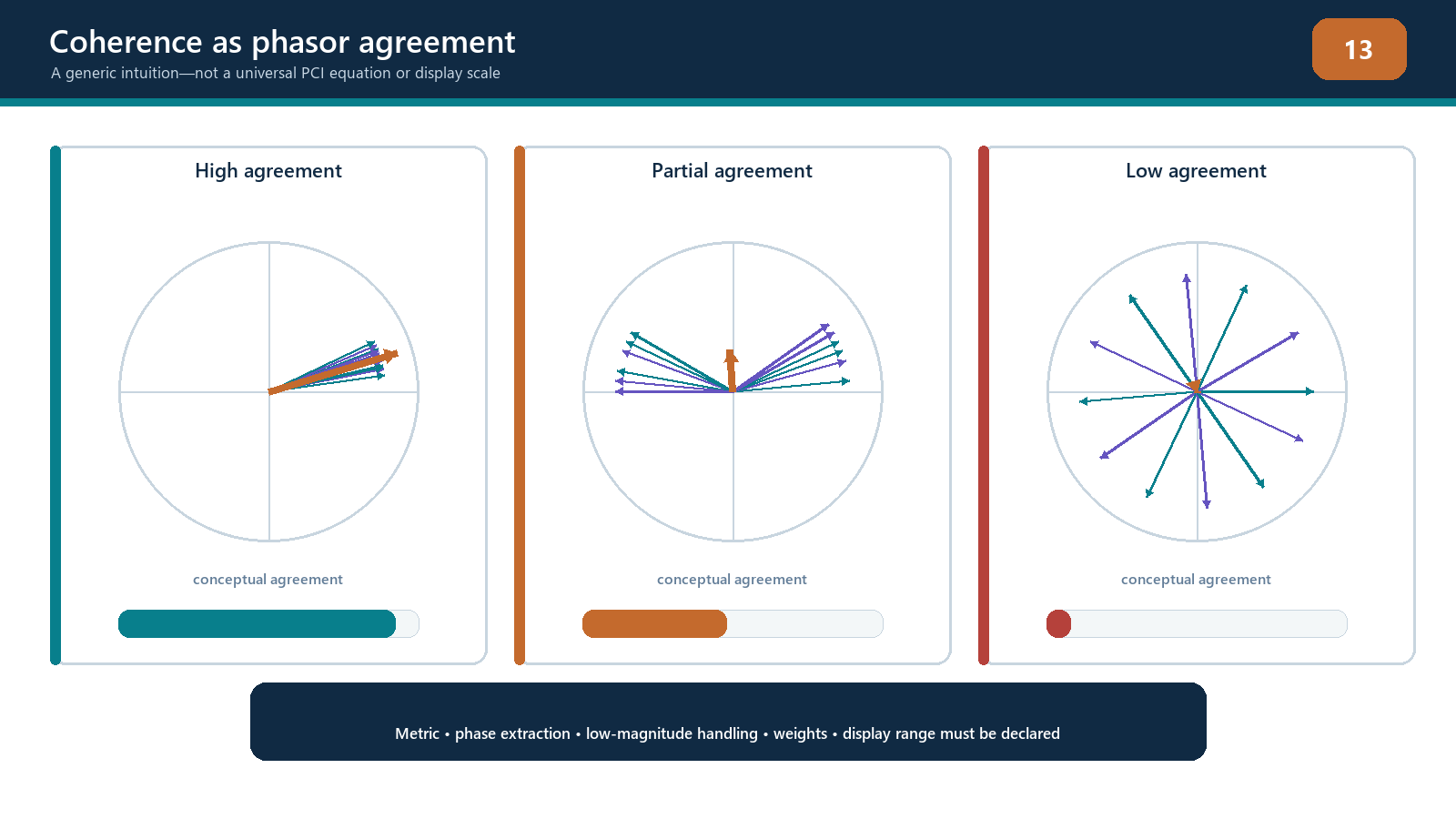
At the correct pixel for a compact reflector and correct path model, many delayed waveforms may reach the same part of the cycle. At a wrong pixel, the delays do not match the event and phases spread. This is the foundation of coherence imaging.
A conceptual vector-coherence score
Let K delayed analytic samples have phase angles φ₁ to φK. Replace each sample by a unit vector pointing at its phase angle, average those vectors and take the length of the result.
C_v = |(1 / K) sum_k exp(i phi_k)|, 0 <= C_v <= 1
The value lies conceptually between zero and one for K > 0. Perfect phase alignment approaches one and perfectly balanced phasors give zero. Random uniformly distributed phases have a non-zero chance resultant for a finite contributor count; the baseline trends toward zero as K increases, with E[C_v^2] = 1/K for independent uniform phases. Amplitude is deliberately removed by using unit vectors.
Important: this equation is a conceptual teaching model only. It is not a description of any particular commercial PCI algorithm. Implementations may use phase standard deviation, sign or polarity, in-phase and quadrature binarisation, different norms, exponents, thresholds, sub-apertures, weighting or normalization. The actual algorithm and output scale must come from controlled implementation documentation.
The conceptual equation also hides practical choices:
Which transmitter–receiver pairs are included?
Is phase evaluated at one sample, over a time window or over frequency?
Are low-amplitude samples rejected before normalization?
Are channel phases corrected?
Is coherence displayed directly or used to weight an amplitude image?
Is the image normalized per frame, per view or to a fixed reference?
Those choices can change the result substantially.
Four evidence conditions
Coherent signal
A real reflector produces signals above noise, the travel-time model is accurate, and many delayed phases agree. Both amplitude TFM and a coherence measure may respond. This is the expected teaching case, but it is not the only coherent case.
Coherent non-defect response
The front surface, backwall, root geometry, sidewall, electrical cross-talk or a repeated instrument transient can be coherent. A coherence image may display it strongly if its timing matches the model. Coherence establishes agreement, not cause.
Phase-inconsistent valid response
A smooth planar reflector can direct energy into only a portion of the receive aperture. Surface roughness, anisotropy, mode mixture or imperfect geometry may vary phase across channels. An amplitude view can show valid energy even when an all-aperture coherence score is weak. Suppression is not proof that the reflector is absent.
Incoherent noise or insufficient signal
Structural and electronic noise with random phase tends to cancel in a coherence calculation. However, when the desired signal is also very weak, the phase estimate is dominated by that noise. A normalized phase-only method cannot manufacture trustworthy phase from no usable acoustic signal.
Timing and model errors
The delay applied to each channel is calculated from geometry and velocity. Consider a true reflector at one coordinate:
a uniform timing offset may shift the apparent position;
an element-dependent delay error spreads phase across the aperture;
wrong specimen velocity produces a depth- and angle-dependent residual error;
wrong wedge velocity or height changes interface timing;
a wrong surface profile changes refraction points;
choosing T instead of L gives a fundamentally wrong time; and
an unmodelled reflection or conversion can align at a false coordinate.
Because phase cycles, a large timing error can occasionally produce local realignment by a whole number of cycles. This may create repeated lobes or ambiguous coherence peaks. Position continuity, amplitude evidence and alternative paths remain necessary.
Bandwidth and frequency dependence
Phase coherence is not independent of frequency. A timing error of 0.05 µs is a quarter cycle at 5 MHz but only one eighth of a cycle at 2.5 MHz. Filtering therefore changes sensitivity to delay error and may change which scattering features dominate.
A broad ultrasonic pulse contains multiple frequencies with different amplitudes and material attenuation. Instantaneous phase can become unstable where the envelope passes near zero or where multiple echoes overlap. The implementation may use a specific band or time window. Record those settings.
Comparing coherence images acquired or filtered at different centre frequencies is not a simple like-for-like comparison. A higher coherence value may reflect the chosen band and model match rather than a more severe discontinuity.
Noise is not always incoherent
Random electronic noise across independent receiver channels is a favourable case for coherence suppression. Field systems also contain:
transmitter breakthrough and cross-talk tied to the firing sequence;
wedge reverberations;
repeated surface ringing;
coherent grain or interface responses;
multiplexing artifacts; and
motion- or coupling-related patterns shared across channels.
These can have repeatable timing and phase. Conversely, real defect responses in coarse-grained or anisotropic material may be distorted differently across paths. The simple statement “defects are coherent and noise is incoherent” is unsafe. The correct statement is that coherence measures phase agreement under a selected model and aperture.
Aperture and sample count
A coherence score based on very few contributing pairs is less persuasive than the same score supported across a broad, physically relevant aperture. Increasing pair count can improve statistical discrimination, but only if the additional pairs contain valid signal and an accurate model. Adding low-directivity or noise-only channels can reduce a real response.
The implementation profile should record:
full or reduced acquisition;
active transmitter and receiver ranges;
sub-aperture rules;
channel exclusions;
minimum valid contributor count;
low-amplitude or quality gating, if documented; and
whether the displayed value is weighted by contributor count.
Without this information, two identical-looking coherence percentages may represent different evidence.
Field workflow: challenge a coherence response
Identify the exact acquisition and coherence implementation.
Confirm the selected path, ROI, aperture, velocity, surface and filter.
Check the source A-scans for adequate unsaturated signal and channel health.
Verify that the response position matches component coordinates and moves correctly with encoded probe position.
Examine phase or delayed RF alignment across representative pairs, not just the displayed score.
Inspect how many elements and pair angles support the response.
Compare the corresponding amplitude TFM or PAUT view on fixed scaling.
Predict coherent geometry echoes and cross-talk times.
Vary one model input within its justified uncertainty and observe response stability.
use a complementary valid path or scan direction;
state whether the evidence supports detection, location, tip interpretation or only further investigation; and
stop if phase is being interpreted without adequate source signal or controlled algorithm information.
Practical 9 — Phase-vector and delay-error experiment
Aim
Observe how phase alignment, timing error and noise affect amplitude summation and a generic vector-coherence score. This is a conceptual experiment, not an emulation of commercial PCI.
Resources
synthetic narrowband bursts with known phase and amplitude;
measured elementary A-scans from a known compact reflector;
a worksheet or script displaying RF, envelope and phasor angles;
a conceptual vector-coherence calculator implementing only the equation in this chapter;
fixed random and coherent-noise examples; and
a record of sampling rate and filters.
Method
Create or load eight equal-amplitude bursts with identical phase. Calculate amplitude sum and conceptual coherence.
Keep phase identical but vary amplitude over a wide range. Note the difference between amplitude sum and unit-vector coherence.
Keep amplitude equal and distribute phase uniformly around the circle.
Create two opposite phase groups and inspect cancellation.
Add random channel noise at increasing levels. Identify when phase becomes unstable.
Add one repeatable coherent transient to all channels. Observe that coherence can remain high for a non-defect event.
Load measured reflector signals and apply their predicted TFM delays.
Introduce controlled delay errors in fractions of the centre-frequency period.
Repeat after a documented filter change and compare sensitivity.
Remove outer-aperture channels, then noise-only channels, recording contributor count.
Compare the conceptual result with the amplitude sum and raw waveforms.
Write one detection statement the evidence supports and one stronger claim it does not support.
Evidence to retain
source waveform set and generation parameters;
phasor plots for aligned, random and opposing conditions;
amplitude-sum and conceptual-coherence table;
delay-error curve with units;
noise and coherent-transient results;
contributor counts and aperture changes;
measured-data comparison; and
a signed statement that the calculation is conceptual, not a commercial algorithm replica.
Stop rules
Stop if source signals are clipped; phase is calculated from an envelope-only export; the sampling or filter is unknown; the conceptual equation is presented as product behaviour; amplitude-near-zero samples are normalized without discussing instability; or a high coherence score is being used alone to classify or accept a flaw.
Common traps
Treating 359° and 1° as widely separated.
Calling polarity the complete instantaneous phase.
Calculating phase from a displayed envelope.
Saying phase is immune to attenuation when the source signal has fallen into noise.
Assuming all repeatable noise is incoherent.
Interpreting a high coherence value as defect severity.
Comparing scores from different apertures or normalisation rules.
Forgetting that high frequency makes a fixed timing error a larger phase error.
Claiming the conceptual vector equation is a commercial PCI algorithm.
Suppressing a valid planar response and concluding the reflector is absent.
Chapter summary
Phase describes position around an oscillatory cycle and must be treated as circular. Correct pixel delays can bring phases from a common event into agreement across many transmitter–receiver pairs. A vector or dispersion measure can describe that agreement, often on a bounded scale.
The generic vector equation in this chapter is conceptual only. PCI and coherence-weighted implementations use different phase, sign, aperture, threshold and normalization rules. Coherence does not prove reflector identity: geometry and cross-talk can be coherent, while valid planar or distorted responses can be phase-inconsistent. Phase also becomes unreliable when source amplitude approaches noise or is clipped. Coherence is strongest when tied back to raw signals, a defensible path model, contributor count and corroborating views.
Study and revision only. This is not an approved inspection procedure, acceptance criterion or qualification.