
CHAPTER 10 · Ultrasonics Level 2
Instrument Controls, Digital Signals and What the Screen Can Hide
In this chapter · 20 sections
Why this matters
A smooth trace can look trustworthy even when useful information has already been lost. The cause may be an overloaded receiver, an unsuitable pulse rate, a gate following the wrong peak or filtering that changes pulse shape. A Level 2 technician does not need to design the electronics, but must understand what each control changes and what the screen cannot recover. This chapter begins with the controls used during a normal examination. It then explains the digital ideas needed to recognise common failures.
What you already need
- The probe returns a changing electrical signal to the instrument.
- Horizontal screen position represents time or a calibrated distance.
- Vertical response height depends on received voltage and gain.
- Pulse length affects axial separation.
- A displayed value is only valid when the correct echo has been selected.
What you will learn
- Explain what range, delay, gain, gate and pulse rate change.
- Distinguish a sampled waveform from the continuous input signal.
- Recognise clipping, ghost responses, aliasing risk and gate-following errors.
- Relate sample interval to distance without calling it resolution.
- Compare filtering, averaging and interpolation by their visible effects.
- Decide which losses can be reprocessed and which require reacquisition.
Words you will meet
- Sample: one measured value of the signal at one instant.
- Sample rate: the number of samples taken each second.
- Clipping: loss of a waveform peak because the receiver range is exceeded.
- Filter: processing that favours some signal frequencies over others.
- Averaging: combining repeated traces to reduce changing noise.
- Interpolation: estimating values between stored samples.
- Pulse repetition frequency: the number of pulse cycles sent each second.
10.1 Start with the controls seen on the instrument
Range selects the time or distance span shown. It must be long enough to include the useful path and any later response needed for interpretation. A short range can hide a back wall. A very long range can compress the useful part of the trace.
Display delay shifts the visible window without changing the physical travel time. It can enlarge a region of interest. It must not be confused with probe zero or wedge delay, which correct a real time contribution before material distance is reported.
Gain amplifies the received electrical signal. It can make a weak response easier to see, but it raises received noise as well. Gain does not improve beam width, pulse length or physical signal-to-noise ratio already present at the receiver.
Gates mark time regions used for alarms or measurements. Gate start, width, threshold and measurement rule affect the reported result. A peak gate and a leading-edge gate can report different times from the same pulse.
Pulse repetition frequency, usually shortened to PRF, controls how often the instrument starts a new pulse cycle. Higher PRF can support faster scanning. If it is too high for the component and path, late energy from one pulse can enter the next trace at a false screen position.
The practical habit is to connect each control to an observable consequence. Moving several controls at once may produce a cleaner display but makes the cause of the change unclear.
10.2 A gate measures by a rule
An automatic number is produced by an algorithm. The instrument may report the first threshold crossing, the highest peak, the crossing nearest a cursor or another feature. That rule matters when pulse shape changes.
Imagine two overlapping echoes. The first is small and the second is large. A leading-edge gate may follow the first response. A peak gate may follow the second. If their relative amplitudes change, the reported position can jump even though neither reflector moved.
Noise can cross a low threshold before the intended echo. Saturation can flatten the top and move the measured peak. A gate placed too narrowly can follow a side lobe or back-wall multiple. The numerical value should therefore be checked against the visible waveform and the declared measurement rule.
10.3 From an analogue voltage to stored samples
The returning electrical signal changes continuously with time. Before it becomes a stored digital trace, an analogue-to-digital converter measures it at regular instants. Each measurement is a sample.
Sample rate states how many samples are taken per second. A rate of 20 million samples per second is written 20 MS/s. The time between samples is the reciprocal of that rate.
In words:
sample interval = one divided by sample rate
| (10.1) Sampling interval · EQ-10-01 Where: Delta_t = time between samples (s); f_s = sample rate (samples/s) Model limits: uniform sampling clock |
|---|
The relationship is useful because a time interval can be expressed as an equivalent pulse-echo distance. The distance is still a sample spacing, not the probe’s resolution.
| Worked example · Express sample spacing as a pulse-echo distance WE-10-01 Given: The sample rate is 20 MS/s. Use a longitudinal-wave speed of 5,900 m/s. Find: The time between samples and the equivalent one-way pulse-echo distance. Steps: Convert the sample rate to samples per second. Delta_t = 1/(20 x 10^6) = 50 x 10^-9 s = 50 ns The pulse travels out and back, so divide its distance by two. Delta_d = c Delta_t/2 = (5,900 m/s)(50 x 10^-9 s)/2 Delta_d = 0.0001475 m = 0.1475 mm Answer: Samples are 50 ns apart, equal to about 0.148 mm of one-way pulse-echo distance. What it means in practice: The waveform is recorded on a 0.148 mm equivalent distance grid. A long pulse or broad beam can still limit physical resolution to several millimetres. Common mistake: Reporting 0.148 mm as the smallest reflector separation the system can resolve. |
|---|
10.4 Sample rate, useful bandwidth and false waveforms
A waveform must be sampled fast enough to represent its useful frequency content. If the rate is too low, a high-frequency component can appear as a false lower-frequency pattern. This effect is called aliasing.
The ideal mathematical boundary is more than two samples for the highest retained frequency. A practical instrument needs extra margin because a probe contains a range of frequencies and real filters do not stop unwanted content at one exact point. Filtering before conversion limits frequencies that could fold into the stored band. [R005]
The figure below shows the same waveform sampled well and poorly. Notice that the sparse samples can form a believable but false pattern.
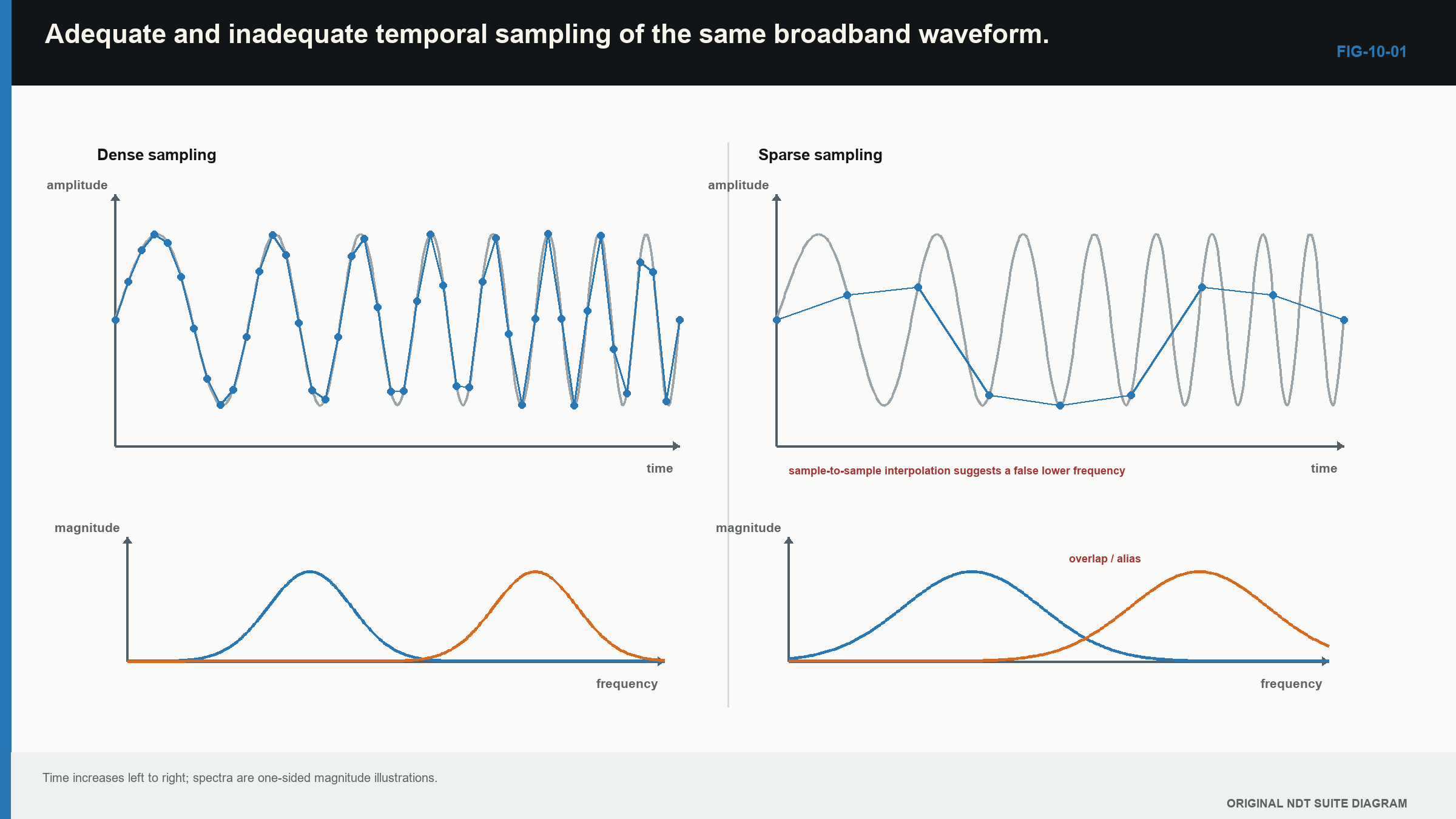
Aliasing is an acquisition loss. A later digital filter sees only the false stored component and cannot know its original frequency. Faster sampling or suitable analogue filtering must prevent the error before it occurs.
10.5 Amplitude range, gain and clipping
Each converter has a limited input range. Receiver gain should place useful echoes well within that range. If the voltage exceeds it, the top or bottom of the waveform is cut off. This is clipping.
A clipped peak may look flat. Increasing gain makes more of the pulse flat rather than taller. Reducing display scale after acquisition only redraws the damaged data. It cannot restore the lost peak, pulse shape or phase.
Too little gain can also waste useful range. A very small echo may occupy only a small part of the available digital levels. More gain can improve its numerical representation if larger echoes remain unsaturated.
| Worked example · Check headroom above a reference echo WE-10-04 Given: Full-scale receiver voltage is 1.0 V peak. A reference echo is 0.50 V peak. A geometry echo may be 8 dB higher. Find: Whether the expected geometry echo remains within full scale. Steps: Convert the 8 dB amplitude increase to a ratio. amplitude ratio = 10^(8/20) = 2.512 expected peak = 0.50 V x 2.512 = 1.256 V Answer: The expected 1.256 V peak exceeds the 1.0 V range and will clip. What it means in practice: The setup needs more headroom if this geometry echo is expected. A reference set at a convenient screen height is not enough if larger production responses overload acquisition. Common mistake: Assuming that reducing the screen height after recording repairs the clipped waveform. |
|---|
10.6 PRF, range and ghost responses
Each pulse needs time to travel through the useful paths and decay before the next cycle creates confusion. If a late echo from the previous pulse arrives after the next pulse has started, it can appear at the wrong range. This is commonly called a PRF ghost or wrap-around response.
A useful diagnostic is to change PRF while leaving probe position, range and coupling unchanged. A genuine component response stays tied to its physical travel time. A wrap-around response often moves or disappears because its position depends on the repetition period.
High PRF also raises average probe loading and can interact with long reverberating paths. The displayed range alone may not show every slow mode or multiple reflection still present in the component.
PRF is not the same as display refresh. The screen can redraw more slowly or use buffering. In array systems, many firings may be required for one complete frame. The relevant acquisition density is the number of complete records stored along the scan, not how lively the display looks.
10.7 Filters change the signal as well as the noise
An analogue filter acts before sampling. It can reduce unwanted frequency content and support anti-alias control. A digital filter acts after sampling. Both can change pulse shape.
A band-pass filter can improve the visible trace when noise lies outside the useful pulse band. It can also remove real signal content, lengthen the pulse or shift the point used for time measurement. A filter change made after calibration may therefore change amplitude and location results.
Envelope detection removes rapid positive and negative oscillation and leaves a smooth magnitude shape. Rectification makes both voltage polarities visible on one side of the baseline. These views are convenient, but they remove polarity information retained by raw radio-frequency data.
Instrument front ends also protect the receiver from the transmit pulse and recover before early echoes arrive. High-voltage excitation, input protection and low-noise reception create practical trade-offs. Published equipment architecture illustrates these functions, although exact values depend on the instrument. [R015]
10.8 Averaging, persistence and motion
Averaging combines repeated traces. Random electronic noise changes from trace to trace, while a stable echo occurs at the same time. Averaging can therefore make the echo easier to see.
The benefit is smaller when the noise is repeatable, such as material backscatter at one position. Averaging also takes time. During scanning, the probe may move across the traces being combined. The result can blur a short indication along the scan direction.
Persistence and peak hold combine information over time for display. They can help a technician see an intermittent response, but the result may not represent one acquisition. The record should show whether these controls affected only the screen or also the stored data.
10.9 Interpolation makes a smoother view, not a richer acquisition
Interpolation estimates values between stored samples or positions. It can make a trace or image easier to read. It can also support more stable timing when the pulse shape is consistent and the method is known.
Interpolation does not add acquired bandwidth. It does not fill a skipped scan line with a real measurement. A display with 0.1 mm pixels may have been built from records 1 mm apart.
This distinction becomes important in encoded scans and later imaging methods. Always separate sample interval, encoded position interval, displayed pixel spacing and physical response width.
10.10 Follow the data from acquisition to result
The instrument can store several different products: raw radio-frequency waveform, filtered waveform, rectified signal, envelope, gated values or a rendered image. Each later product depends on earlier information.
The next figure shows the branches. Notice that clipping and aliasing happen before later processing can repair them. A value-only export can also remove the waveform needed to check echo identity.
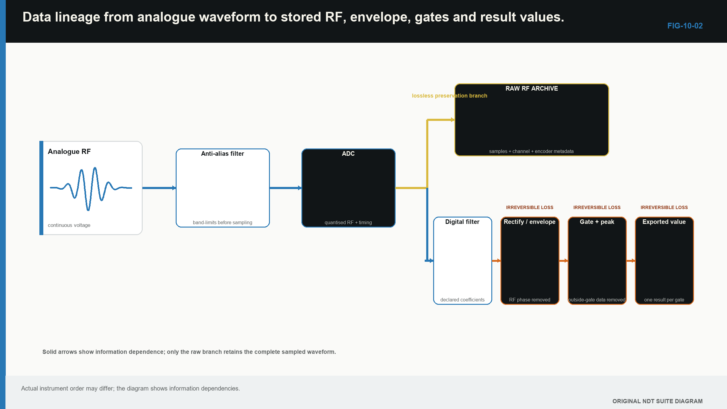
Some changes can be revisited when raw data and metadata survive. A different digital filter, envelope or display scale may be applied later. Missing records, clipped peaks and aliased frequencies normally require reacquisition.
The practical test is simple: processing can reorganise stored information, but it cannot recreate information that never entered the data. Conventional instrument principles remain tied to the same pulse, path and A-scan, the time-amplitude waveform used throughout UT. [R001]
In plain words
- Range and delay control what part of the trace is shown.
- Gain changes electrical response height, not beam width or physical resolution.
- A gate reports a value by a chosen timing or amplitude rule.
- Sample interval is a digital grid, not a statement of physical resolution.
- Clipping and aliasing destroy information during acquisition.
- Filtering and averaging can help visibility while changing pulse shape or spatial detail.
- Interpolation makes the display smoother without adding new measurements.
- Raw data and settings determine which later questions can still be answered.
Key terms
- Sample: one digital measurement at one time.
- Sample rate: samples taken per second.
- Clipping: loss caused by exceeding the receiver range.
- Aliasing: false lower-frequency content caused by inadequate sampling control.
- Gate: a selected trace region used for an alarm or measurement.
- PRF: the number of pulse cycles started per second.
- Interpolation: estimation between stored values.
Key relationships
- Delta_t = 1/f_s converts sample rate into time between samples.
- Delta_d = c Delta_t/2 expresses that interval as equivalent pulse-echo distance.
- amplitude ratio = 10^(dB/20) converts an amplitude change in decibels to a ratio.
Common mix-ups
- Gain is not physical signal-to-noise improvement.
- Sample spacing is not axial resolution.
- PRF is not display refresh rate.
- A smooth interpolated line is not a continuously measured signal.
- A smaller display scale cannot repair clipping.
Bridge to Chapter 11
Chapter 10 explained how the instrument can preserve or lose information. Chapter 11 returns to the acoustic side of the system. It shows how the target, access, surface and required result guide the choice of probe and transmission arrangement.
Sources and further study
- [R001]
- [R005]
- [R015]
Study and revision only. This is not an approved inspection procedure, acceptance criterion or qualification.