
CHAPTER 19 · Ultrasonics Level 3
When the Simple Wave Model Stops Working
In this chapter · 22 sections
Why this matters
A Level 2 technician normally treats one wave mode as travelling at one velocity along a predictable refracted path; that model works well in many fine-grained, nearly uniform components. It becomes unreliable when a beam splits, a target plots in the wrong place, velocity changes with direction, or useful response disappears inside a textured weld. Level 3 work begins with those visible symptoms. The aim is not to begin with advanced stiffness mathematics. It is to recognise which assumption failed, select a better level of model and demand physical evidence before trusting the more complicated prediction.
What you already need
- Longitudinal and shear-wave motion in an approximately isotropic solid.
- Wavelength, frequency, velocity and the basic refraction picture.
- Familiarity with angle-beam paths, beam width and target orientation.
- The practical difference between loss of signal and movement of a beam.
- Basic trigonometry and exponential or decibel loss calculations.
What you will learn
- Diagnose symptoms caused by directional, dispersive or heterogeneous propagation.
- Explain isotropic and anisotropic behaviour without starting from advanced algebra.
- Distinguish wavefront direction, energy direction and polarisation.
- Separate absorption, scattering, beam spread, redirection and interface loss.
- Choose among ray, beam, measured-field and full-wave evidence.
- State when advanced wave mathematics belongs in the Part VIII engineering treatment.
Words you will meet
- Isotropic: having the same relevant wave behaviour in every material direction.
- Anisotropic: having wave behaviour that depends on material direction.
- Wavefront: a surface whose points share the same wave phase.
- Phase direction: direction normal to a wavefront.
- Group direction: direction in which a narrow wave packet and its energy commonly travel.
- Polarisation: direction and pattern of particle motion for a wave mode.
- Slowness: reciprocal of phase speed, used to show directional wave behaviour.
- Dispersion: change of phase or group behaviour with frequency.
- Structural noise: received field created by scattering from material structure.
- Model discrepancy: remaining difference between model and reality after inputs are considered.
Depth guide for this chapter
- Understand here: symptoms, direction concepts, model limits and evidence selection.
- Calculate here: path-coordinate bias, effective attenuation and pulse-spread bounds.
- Derive later: directional-stiffness mathematics, formal mode solving, slowness construction and full-wave equations are developed in Chapters 64 to 66 and Chapter 70.
19.1 Start from the Level 2 symptoms
The simple model assumes a homogeneous material, one effective mode, a scalar velocity and geometry that changes slowly compared with wavelength; its beam is finite, but its centreline is normally treated as predictable. Four common symptoms show that this picture needs attention. A split beam produces two or more strong regions where one was expected; a wrong location occurs when repeatable time data map to an implausible coordinate. Direction-dependent velocity appears when nominally equivalent paths give different transit behaviour after geometry and zero are controlled. Lost signal occurs when a known target or far surface cannot be recovered with the expected signal-to-noise.
Each symptom has several possible causes; a lost signal can result from absorption, scattering, beam redirection, defocusing, mode conversion, poor coupling or receiver recovery. A wrong location can arise from velocity, angle, index, coordinate registration or echo identity. Level 3 diagnosis compares observables that divide those explanations. Adding gain before identifying the mechanism can create a busier screen while leaving the missing evidence missing. The first diagnostic step remains practical; map the response over probe position, compare opposite directions, examine spectral change, use an electrical or simple acoustic reference, and compare a known target through representative material. The formal model is added only when the observations show which simplification failed.
19.2 Isotropic and directional behaviour
In an isotropic model, the relevant elastic response is the same in every direction; a longitudinal-wave speed and a shear-wave speed can represent common bulk propagation. Two shear polarisations share the same speed in an ideal isotropic solid. The familiar refraction diagram is built on this simplification. An anisotropic material responds differently with direction; texture, oriented dendrites, crystal structure or laminate architecture can make phase speed and particle motion direction-dependent. The material can support quasi-longitudinal and quasi-shear modes. The word quasi means that the motion is mainly, but not exactly, parallel or perpendicular to the phase direction.
This distinction is visible before it is mathematical; rotating a specimen or changing scan direction can change arrival time, beam position, mode content or attenuation. In a composite, changing ply direction changes the relationship between wavefront and energy flow. In an austenitic weld, local dendritic orientation can vary across passes, so one uniform directional model may also be insufficient. United States National Aeronautics and Space Administration (NASA) analytical ultrasonics work describes quasi-modes, phase and group directions, and multiple transmitted modes in composite media. [R006] Work on austenitic welds likewise treats anisotropy and scattering as central to the examination problem. [R008] These sources support the need for a direction-aware model; they do not give one universal material description for every component.
19.3 Wavefront direction, energy direction and polarisation
A wavefront connects locations at the same phase; its normal defines the phase direction, represented by the wave vector. The group direction describes how a narrow packet moves through a medium and commonly follows the direction of energy transport in a lossless case. In an isotropic material these directions align. In an anisotropic material they can separate. This separation explains a familiar field problem; refraction at an interface can satisfy phase matching while the main energy travels away from the line drawn using isotropic Snell’s law. A measured transit time may remain repeatable while the reflector location is biased. More timing precision cannot correct the wrong directional model.
Polarisation describes particle motion; it controls how the source excites a mode, how boundary conditions divide energy between modes and how the wave interacts with a target. The same nominal angle does not guarantee the same target response when mode or polarisation changes. A longitudinal arrangement may penetrate a particular weld better than a shear arrangement, but that tendency still needs evidence for the actual direction, texture, frequency and target.
A slowness surface plots reciprocal phase speed against direction; in a two-dimensional section, the radius indicates phase slowness and the normal indicates group direction under the usual lossless interpretation. The following figure shows the geometry. Notice that the anisotropic normal is not generally collinear with the radius.
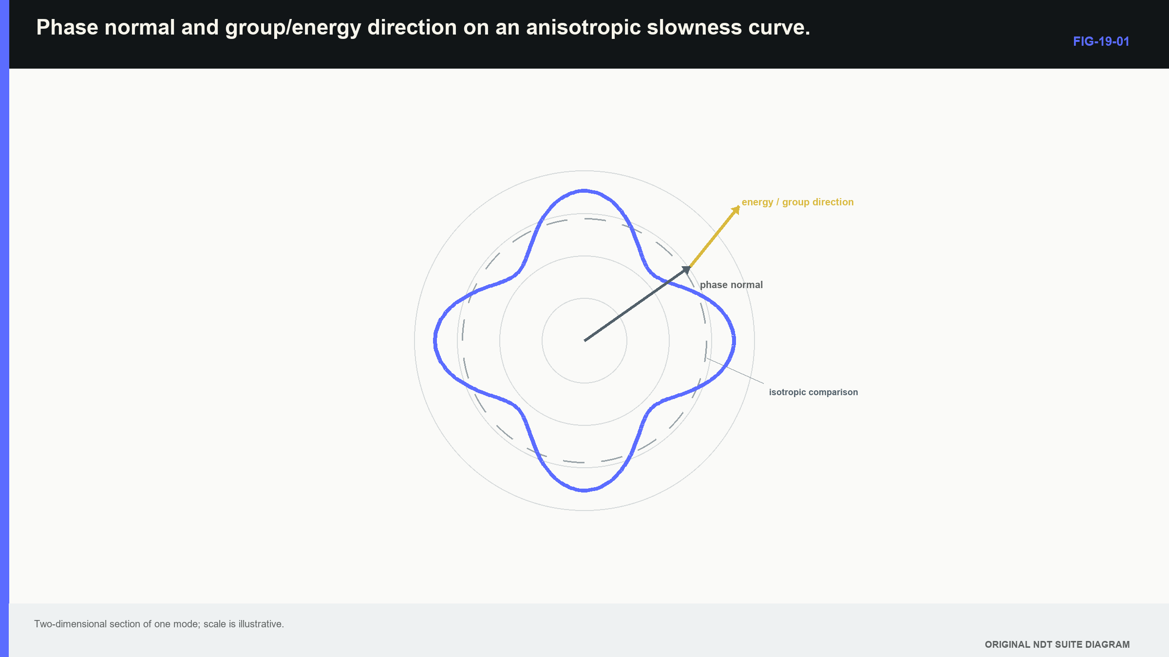
Flat or strongly curved parts of a slowness surface can concentrate, spread or divide energy; a Level 3 reader should be able to interpret that consequence from a supplied plot. Construction from stiffness data and formal differentiation are Part VIII tasks.
19.4 Technical decision case: a precise echo in the wrong place
| Worked example · Location bias from an unmodelled group direction WE-19-01 Given: A model assumes energy travels 45.0 degrees from normal over a 60.0 mm path. The actual group direction is 50.0 degrees while measured path length is otherwise correct. Find: The modelled and actual horizontal offsets and depth components. Steps: For the model, x = 60 sin45 = 42.43 mm and z = 60 cos45 = 42.43 mm. For the actual energy direction, x = 60 sin50 = 45.96 mm and z = 60 cos50 = 38.57 mm. Subtract model coordinates from actual coordinates. Answer: Horizontal location is biased by +3.53 mm, and depth is biased by -3.86 mm. Technical implication: A five-degree directional-model error creates millimetre-scale coordinate error even when transit time is measured precisely. Coverage and location evidence must represent the energy direction. Common mistake: Improving cursor precision or adding decimal places cannot remove bias caused by the wrong propagation direction. |
|---|
This case separates calculation from derivation; the Level 3 calculation uses supplied directions and basic trigonometry. The derivation of those directions from elastic constants is deliberately deferred to Chapter 65.14 and Chapter 66.1.
19.5 Dispersion, absorption and apparent attenuation
Dispersion means wave speed or group behaviour varies with frequency; common bulk waves in a homogeneous elastic continuum can be approximately nondispersive across an NDT band. Guided waves, layered materials and viscoelastic media can be strongly dispersive. A finite pulse then reshapes because different frequency components accumulate different phase and delay. Attenuation must be divided into mechanisms. Absorption transfers coherent acoustic energy into heat or internal material motion. Scattering redirects energy through interaction with heterogeneity; geometric spreading, beam defocusing and interface transmission also reduce a measured amplitude, but they are not material absorption. Calling every decrease “attenuation” without controlling the field can assign the wrong cause.
Over a limited range, an effective exponential model can describe amplitude loss.
| (19.1) Exponential amplitude-loss model · EQ-19-02 Where: A = amplitude after distance x; A_0 = amplitude at reference position; alpha = amplitude attenuation coefficient (Np/m); f = frequency (Hz); x = path length (m) Model limits: one effective mode in a homogeneous path; separates neither beam spread nor interface loss unless controlled experimentally |
|---|
The observable is amplitude change across a controlled path; the model can support a comparison between frequencies or distances when geometry, field and interfaces are comparable. It does not identify absorption separately from unrepresented loss. For an amplitude coefficient in nepers per metre, the corresponding decibel amplitude change is -8.686 alpha x.
| Worked example · Frequency-dependent loss over a pulse-echo path WE-19-02 Given: Effective amplitude attenuation is 0.8 dB/mm at 5 MHz and 0.25 dB/mm at 2 MHz for one controlled material and path comparison. One-way distance is 30 mm, making the pulse-echo material path 60 mm. Find: Relative path loss at each frequency, excluding separate beam and interface effects. Steps: Multiply each declared coefficient by the 60 mm total path. At 5 MHz, loss is 0.8 x 60 = 48 dB. At 2 MHz, loss is 0.25 x 60 = 15 dB. Their difference is 33 dB. Answer: Effective loss is 48 dB at 5 MHz and 15 dB at 2 MHz under the stated comparison. Technical implication: Lower frequency has a strong penetration advantage in this case, although its longer pulse and wider field may reduce resolution. Common mistake: Transferring these coefficients to another material, direction or setup treats an empirical system result as a universal material constant. |
|---|
Frequency-dependent loss can shift the effective centre frequency lower with distance; the received pulse can therefore be longer than the emitted pulse and can move the timing feature selected by an algorithm. Timing method becomes part of the measurement definition.
19.6 Wave packets and resolvability
A real pulse contains a band of frequencies; carrier phase travels at phase velocity, while the envelope of a narrowband packet travels approximately at group velocity. When dispersion is weak over a short path, the difference may not be visible. When dispersion is strong, the packet broadens and its peak changes shape. The formal group-velocity relationship is shown here for recognition and use with a supplied dispersion curve.
| (19.2) Group velocity · EQ-19-03 Where: v_g = group-velocity vector (m/s); omega = angular frequency (rad/s); k = wave vector (rad/m) Model limits: differentiable dispersion relation and wave packet sufficiently narrow in wave-number space |
|---|
This equation supports interpretation of arrival direction and packet delay; Part III does not require the learner to calculate a multidimensional gradient from first principles. Chapter 64 teaches derivatives and fields, while Chapters 66.2 and 66.15 develop group velocity and dispersive wave packets.
| Worked example · Estimating pulse broadening from group-delay variation WE-19-03 Given: Across the useful bandwidth of a guided mode, calculated group delay over the inspection distance ranges from 82 microseconds to 91 microseconds. The emitted envelope duration is 4 microseconds. Find: A first bound on temporal spread caused by dispersion. Steps: Subtract the earliest group delay from the latest: 91 - 82 = 9 microseconds. Compare that range with the 4 microsecond emitted duration. Answer: Delay variation alone spans 9 microseconds, which exceeds the emitted duration. The received packet can be much broader than the original pulse. Technical implication: A narrow gate at the nominal arrival can exclude useful energy or merge neighbouring modes. Exact waveform prediction needs spectral weighting and phase. Common mistake: Treating the 9 microsecond bound as the exact final pulse duration ignores the source spectrum and complete system response. |
|---|
Dispersion curves can contain several branches and turning regions; a favourable frequency-thickness point for one mode can also support unwanted modes. Mode identity should use arrival trends, frequency content and field behaviour together.
19.7 Scattering and structural noise
Scattering strength depends partly on heterogeneity scale relative to wavelength; when grains or structural features are much smaller than wavelength, an effective-medium model may work. As scales become comparable, scattering and mode conversion increase. Large planar boundaries produce directional reflection, while distributed structure produces a speckle-like field. Structural noise is not electronic noise simply added after the target signal; it is an acoustic field created by many scatterers with different phases. Moving the probe by a fraction of a wavelength can change the interference pattern. Averaging genuinely different positions may reduce some random components, while averaging highly correlated samples mainly smooths the display.
Material-characterisation research also shows that velocity and backscatter can respond to microstructure while remaining dependent on controlled models, calibration and field conditions. [R009] Target and structure can also interfere coherently; a weak reflector can reinforce the local background at one position and cancel it at another. One signal-to-noise ratio then gives an incomplete description. Distributions across position, orientation and material can be more useful for detection evidence.
Ultrasonic material-characterisation research shows that velocity and backscatter respond to microstructure, but the inverse relationship is not unique; grain size, texture, phase fraction, elastic contrast, field and bandwidth all contribute. [R009] A single effective attenuation or backscatter number should not be reported as a unique microstructure measurement without a validated model.
19.8 Layers, curvature and interfaces
At a planar interface, phase matching preserves tangential wave number; boundary conditions connect displacement and traction and determine reflected and transmitted modes. Path direction may be predicted reasonably while amplitude remains uncertain because amplitude also depends on polarisation, conversion coefficients, source spectrum, loading, interface condition and target response. Energy conservation is a useful check for an ideal lossless calculation, but a displacement-amplitude coefficient cannot simply be squared and interpreted as energy; energy flux includes stress, particle velocity and energy-flow direction. Roughness or material loss can also move energy out of the coherent measured mode.
Thin layers can resonate or interfere; curvature changes local incidence and can focus or defocus a finite beam. Roughness supplies a distribution of local surface normals and increases diffuse scattering as its scale approaches wavelength. A two-dimensional central ray can therefore look correct while the actual field loses coverage. This creates a hierarchy of amplitude claims; a validated path model can support geometry. Relative amplitude trends require tighter source, receiver, field and target control. Absolute amplitude prediction needs a much more complete validated system. Elegant boundary equations do not erase uncertain material and surface inputs.
19.9 Austenitic welds as a coupled problem
An austenitic weld can combine anisotropy, heterogeneous orientation, attenuation, scattering, curvature of fusion boundaries and strong geometry responses; the beam may skew, broaden or split. Different quasi-modes may overlap. One average velocity can match one reference and mislocate another path. A defensible examination can use macrostructure-informed path models, lower frequency, longitudinal modes, access from more than one side, measured fields and representative specimens; no single item is automatically sufficient. A generic weld texture used in a sophisticated simulation remains an uncertain assumption until compared with actual field or target evidence.
Opposite directions are especially informative; agreement in coordinates across physically different paths can strengthen a hypothesis. Disagreement can reveal material-direction effects. A response present in only one configuration is not automatically false; each mode and path illuminates a different orientation and passes through different material. The technical decision should name the capability region; some paths may support detection but not sizing. Other areas may remain unexamined because structural noise prevents a stable reference. A bounded limitation is more useful than converting a missing interpretable echo into evidence of no discontinuity.
19.10 Choosing the required model
A model hierarchy helps avoid both under-modelling and decorative complexity:
- Scalar velocity and central rays test simple path plausibility.
- Beam models add aperture, diffraction, width and focusing.
- Directional ray or measured-field models add anisotropic path effects.
- Semi-analytical models add selected wave and interface behaviour.
- Full numerical elastodynamics represents complex fields, scattering and boundaries.
The controlling error mechanism sets the level; access geometry may need only a ray with measured angle. Coverage across a focal region needs a beam. Strong splitting in a heterogeneous weld may justify numerical or experimental field mapping. More model detail without reliable stiffness, attenuation, texture or geometry can produce a precise representation of poor assumptions. Verification establishes that equations or software were solved correctly; validation establishes that the chosen physics represents reality adequately for the intended output. Analytical limits, convergence and energy balance support verification. Travel-time, field-map and target-response comparisons support validation. A time match does not automatically validate amplitude.
Sensitivity analysis identifies influential uncertain inputs; local derivatives are efficient near smooth behaviour. Global sampling is safer around mode switching, caustics or thresholds. Arrival time, beam coverage, peak amplitude and detectability can have different dominant inputs. The output used in the sensitivity study must match the technical decision. The open continuum-wave foundation used by the later engineering chapters is represented in the cited wave-mechanics source. [R004] Full sensitivity, simulation and model-discrepancy treatment continues in Chapters 66.17 to 66.20 and Chapter 70.
19.11 Formal model boundary and forward route
An eigenproblem is a formal calculation that finds allowed values together with their associated directions. The Christoffel eigenproblem is the formal route from anisotropic stiffness and direction to allowed phase speeds and polarisations. A stiffness tensor is a structured collection of material constants that represents how elastic response changes with direction.
| (19.3) Christoffel eigenproblem · EQ-19-01 Where: Gamma_ik = C_ijkl n_j n_l; C_ijkl = stiffness tensor (Pa); n = unit wave-normal vector; rho = density (kg/m^3); c_p = phase speed (m/s); p = polarisation eigenvector; delta = identity tensor Model limits: homogeneous linear elastic anisotropic medium and plane harmonic wave |
|---|
At Level 3, this equation is a map of dependencies; material stiffness C, density rho and wave-normal direction n determine permitted phase speeds and polarisation vectors. The observable consequences are directional velocity, mode content, beam skew and target interaction. The learner is not expected to assemble a fourth-order tensor or solve the eigenproblem here. The complete route is explicit:
- Chapter 64.6 introduces eigenvectors and the information carried by matrix problems.
- Chapters 65.1 to 65.4 develop stress, strain, constitutive response and wave equations.
- Chapter 65.14 derives a plane wave in an anisotropic solid.
- Chapter 65.18 treats tensor rotation and material frames.
- Chapters 66.1, 66.2 and 66.8 develop the Christoffel problem, group direction and slowness surfaces.
- Chapter 70 develops numerical simulation, verification and validation.
Part III uses the engineering consequences now and reserves the full derivation for the mathematical destination prepared for it.
In plain words
- The simple scalar-velocity model remains useful until its assumptions fail visibly or materially.
- Beam splitting, wrong location, directional velocity and lost response are model-breakdown symptoms.
- In directional materials, wavefront direction and energy direction may not align.
- Polarisation changes excitation, mode conversion and target response.
- Measured amplitude loss can combine absorption, scattering, beam spread, redirection and interface effects.
- Dispersion changes pulse shape and can make timing depend on the selected waveform feature.
- Model complexity should increase only when a simpler model cannot support the decision.
- Verification checks the solution; validation checks whether the physical model is adequate.
Key terms
- Isotropic: same relevant response in every material direction.
- Anisotropic: response varies with material direction.
- Phase direction: normal direction to the wavefront.
- Group direction: packet and common energy-transport direction.
- Polarisation: particle-motion pattern of the mode.
- Slowness: reciprocal phase speed represented by direction.
- Dispersion: frequency-dependent phase or group behaviour.
- Structural noise: acoustic field scattered by material structure.
- Model discrepancy: residual difference between model and reality.
Key relationships
- A = A_0 exp(-alpha x): effective exponential loss applies only within its controlled path and mode assumptions.
- v_g = grad_k omega(k): group velocity follows the gradient of the dispersion relationship.
- (Gamma - rho c_p^2 I)p = 0: anisotropic stiffness and direction determine allowed phase speeds and polarisations.
- model level -> observable error mechanism: the decision determines required complexity.
Common mix-ups
- Phase direction is not always the energy direction.
- A lower echo is not proof of greater material absorption.
- Structural noise is not merely electronic receiver noise.
- A verified simulation is not automatically validated for the component.
- Precise transit time does not guarantee correct coordinates under the wrong path model.
Bridge to Chapter 20
Chapter 19 showed that material and field behaviour can move, broaden or reshape an ultrasonic response; chapter 20 turns that insight toward the probe and assembled system. It begins with two nominally identical probes that produce different screens and establishes which measured properties control substitution.
Sources and further study
- [R004]
- [R006]
- [R008]
- [R009]
Study and revision only. This is not an approved inspection procedure, acceptance criterion or qualification.