Coordinates, Offsets, Skew and Scan Patterns

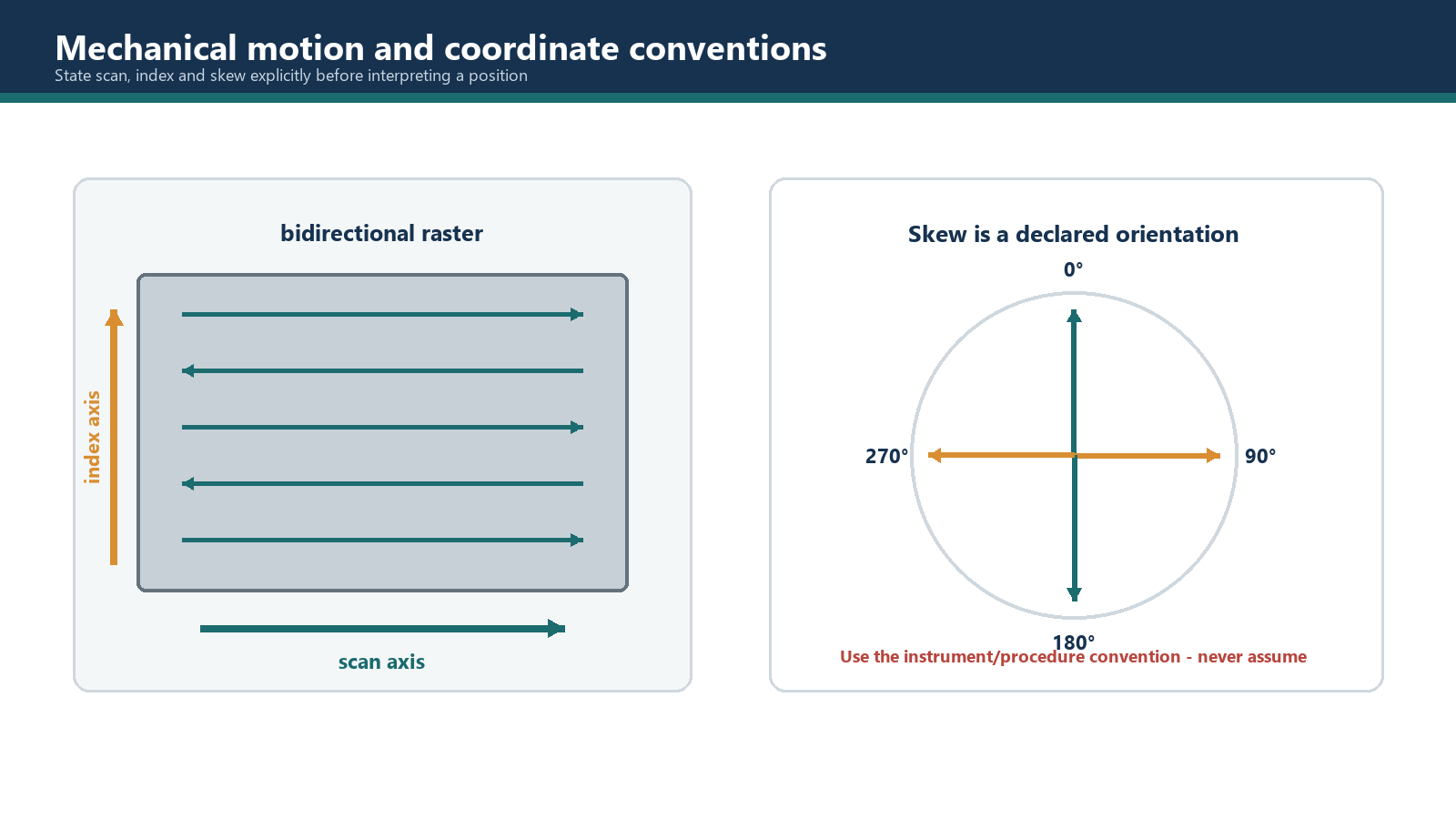
This chapter establishes the spatial language used to plan and record probe movement. Its purpose is to ensure that a beam, a probe path and a stored indication can be related to the same component datum without relying on an unlabelled sketch or an instrument's default axis names.

Learning outcomes

After completing this chapter, the learner should be able to:

1. establish a component-based origin and positive coordinate directions;
2. distinguish scan, index and through-thickness coordinates;
3. define scan and index offsets from an identified mechanical or acoustic reference point;
4. distinguish skew from refracted angle and declare the selected angular convention;
5. describe one-line, skewed, unidirectional and bidirectional raster paths;
6. describe spiral, helical and complex-shape paths without assuming a universal axis convention;
7. calculate raster line positions using an inclusive endpoint convention;
8. identify how overlap, access, overrun, direction reversal and component geometry affect a scan plan;
9. produce a scan-pattern record that another operator can reproduce.

Key terms

Component datum: A physical feature, mark or defined geometry from which positions are measured.

Origin: The point assigned zero values in the selected coordinate system.

Scan axis: The primary coordinate direction along which data are collected during one scan line.

Index axis: The coordinate direction used to separate adjacent scan lines or probe positions.

Through-thickness coordinate: Position measured into or through the component using a declared surface and sign convention.

Scan offset: The signed scan-axis distance between a defined reference and the acquisition origin.

Index offset: The signed index-axis distance between a defined reference and the acquisition origin or probe reference position.

Skew: A plan-view orientation angle measured from a declared zero direction using a declared positive sense.

One-line path: Probe movement along one scan line at a nominally fixed index position.

Raster: A set of substantially parallel scan lines separated by controlled index steps.

Unidirectional raster: A raster in which data are acquired in the same scan direction on every line.

Bidirectional raster: A raster in which data are acquired on alternating forward and reverse lines.

Spiral path: A path that changes angular position and radius around a defined centre.

Helical path: A path that combines rotation around a cylindrical or similar surface with translation along its axis.

11.1 Establish the coordinates before drawing the path

A scan plan begins with the component, not with the scanner. Identify a stable datum that can be found during setup, acquisition and later review. Examples include a weld centreline, machined edge, nozzle centreline, pipe clock position or a permanently marked survey point. A painted line with no dimensional relationship to the component is only a guide, not a datum.

The coordinate definition must state:

• the origin and the physical feature that realises it;
• the scan and index axes;
• the positive direction of each axis;
• the surface or local geometry from which depth is measured;
• units and angular convention;
• the probe, wedge or scanner reference point used for offsets;
• whether coordinates follow a flat plane, cylinder, developed surface or three-dimensional model.

Axis labels such as X and Y are convenient but not self-explanatory. One instrument may assign X to the scan encoder, another may call that axis Y, and a CAD model may use both differently. The technique should define functional names first and then map them to equipment channels.

11.2 Scan, index and depth coordinates

The scan axis is normally the direction in which one acquisition line progresses. For a long weld, this may run parallel to the weld. For a circumferential pipe scan, it may follow the developed circumferential direction. The name describes the inspection coordinate, not necessarily a global horizontal direction.

The index axis separates neighbouring scan lines, passes or probe positions. In a plate raster it is commonly perpendicular to the scan axis. In a complex geometry, the index path may follow a surface curve and need not be a straight Cartesian axis.

The through-thickness coordinate describes position into the component. It may be called depth when measured normal to a reference surface, but a sloping, curved or layered component requires care. Sound path, vertical depth and surface-projected position are different quantities. Chapter 5 explains how corrected displays use geometry to present these values.

Scan and index coordinates describe movement on or related to the surface. Refracted angle describes beam direction in a section through the material. Skew describes the plan-view orientation of the probe or beam plane. Keeping those roles separate prevents an angular setting from being entered on the wrong axis.

11.3 Reference points and signed offsets

A scanner encoder measures movement from its zero; it does not know where the weld or component datum is. An offset connects the scanner or probe reference to the component coordinate system.

Possible mechanical references include a scanner wheel centre, a carriage mark, the front edge of a wedge or a dedicated survey point. Possible acoustic references include a nominal beam exit or index point. The two are not automatically the same. In an electronic linear sequence, the acoustic index position may change with the active aperture while the scanner reference remains fixed.

A useful offset states the named datum, the named probe/scanner reference, the axis and the sign. For example: "At scan zero, wedge mark W1 is at S = -25 mm and I = +42 mm relative to the weld-centreline origin." The note "offset 42" is not reproducible.

Software may define offset in the opposite direction, such as datum-to-probe rather than probe-to-datum. Confirm the entry convention using a known point and review the corrected coordinates before production acquisition. A numerically plausible image can still be mirrored or shifted when a sign is wrong.

11.4 Skew requires a declared convention

Skew is measured in plan view. It is not the refracted angle measured from the surface normal. Rotating an angle-beam wedge on the surface changes the beam plane's plan-view orientation even if the refracted angle within that plane remains nominally the same.

For examples in this chapter only, use this course convention:

• 0 degrees points along +S;
• 90 degrees points along +I;
• 180 degrees points along -S;
• 270 degrees points along -I;
• positive skew is measured clockwise when looking toward the test surface from above.

This convention is not universal. Some instruments measure counterclockwise, use a different zero, show signed angles from -180 to +180 degrees or define probe orientation instead of beam projection. A procedure must state its convention and the setup must be checked against a physical reference direction.

For a one-dimensional linear array, the electronically steered beam normally remains in the active plane fixed by the array and wedge orientation. Mechanical rotation of the probe changes the skew of that plane. A suitable matrix or laterally segmented array may steer in skew electronically, but the law record must distinguish electronic skew from physical probe rotation.

11.5 One-line and skewed paths

A one-line path moves along the scan axis at a nominally fixed index position. Record start, end, direction, index, probe orientation and overrun. Overrun is required when the sound field is displaced from the encoder reference; stopping the wheel at a boundary may leave the beam short of it.

A skewed path is not aligned with the principal scan axis. Define it by start/end coordinates or a path angle, and ensure the encoder measures travel in that direction without side slip. Path direction and beam skew are separate vectors and both belong in the plan.

11.6 Raster patterns

A raster covers an area using a series of adjacent lines. The line spacing is the index increment. The required spacing comes from the verified effective coverage width, target orientation, surface geometry and any procedural maximum. It is not chosen solely because an encoder can resolve a small distance.

Unidirectional raster

In a unidirectional raster, every acquired line runs in the same scan direction. After a line is completed, the probe returns without acquiring, indexes to the next position and begins again from the same side.

Potential advantages include consistent mechanical loading, cable pull, wheel direction and probe orientation. It can reduce direction-reversal effects in scanners with backlash or asymmetric coupling. The cost is extra return travel and time. The return path must not accidentally overwrite or append data to the previous line.

Bidirectional raster

In a bidirectional raster, data are acquired in both directions. At the end of one line, the probe indexes and scans the next line in reverse. This reduces non-acquiring return travel, but forward and reverse behaviour must be shown to be equivalent.

Check encoder backlash, wheel slip, carriage play, cable drag, couplant delivery and any direction-dependent probe tilt. The software must associate each line with its true coordinate direction; simply reversing the display can hide a polarity error.

Neither pattern is inherently superior. The qualified scanner and component conditions decide which one gives reliable coverage and position accuracy.

Worked example 11.1 - planning a bidirectional raster

Given: A rectangular inspection region extends from S = 0 mm to S = 220 mm and from I = 0 mm to I = 64 mm. A qualified setup permits an 8 mm index step. Both index boundaries must be included.

Assumptions: The effective coverage width has been verified as at least 12 mm under the inspection conditions; the component is flat; the scanner can acquire equivalently in both scan directions; required approach and exit overruns are documented separately.

Line positions: Starting at 0 mm and stepping by 8 mm gives index positions 0, 8, 16, 24, 32, 40, 48, 56 and 64 mm. There are nine acquired lines.

Nominal overlap: A 12 mm verified coverage width and 8 mm line spacing provide 4 mm nominal overlap between adjacent coverage strips. This is a planning value; coupling and edge response still need verification.

Path: Line 1 runs from S = 0 to S = 220 mm. The scanner indexes to I = 8 mm; line 2 returns from S = 220 to S = 0 mm. Direction alternates until line 9 is complete.

Acquired travel: Nine lines of 220 mm produce 1,980 mm of acquired scan travel, excluding index moves, approach, exit and repositioning.

Verification: Confirm the first and last coverage strips extend to both region boundaries, check forward/reverse coordinate polarity and verify no line was missed or repeated.

11.7 Spiral paths

A spiral combines rotation around a centre with changing radius. Define centre, start radius, rotation sense, radial change per revolution, probe orientation and end condition. Surface speed and turn overlap can change with radius, so check rate and spacing over the complete path. The probe footprint may leave an uncovered centre or outer edge; address those areas with a supplementary path.

11.8 Helical paths on cylindrical components

A helix combines circumferential rotation with axial translation. Record whether circumferential position uses distance, angle or counts; define axial direction, pitch, start clock position, rotation sense, overlap and probe orientation.

A developed cylindrical map has a 0/360-degree display seam. Confirm continuity in the underlying coordinates and physical closure of the path. A split display is not necessarily a coverage gap, while an unscanned closure strip is.

11.9 Complex surfaces and multi-axis paths

Nozzles, elbows, branches and contoured products may need several axes. Control the geometry model and revision, component alignment, local surface normal, probe contact point and orientation, axis calibration, coupling limits and coordinate transformation. A robot can report its joints precisely while the acoustic coordinates remain wrong because its tool centre or surface model is wrong.

Use controlled drawings, survey data or qualified surface mapping; do not infer unmeasured dimensions from a photograph. Revise the plan or record the limitation when the real surface departs enough to affect contact or beam paths.

11.10 Overlap and coverage boundaries

Overlap is the shared verified coverage between adjacent passes, not merely the distance between central rays. Establish the useful beam region for the target class and depth range, then place mechanical paths so that those regions cover the required volume.

Coverage may be reduced at:

• start and end positions where the probe cannot overrun;
• first and last electronic apertures;
• extreme sector angles;
• curved-surface edges where coupling changes;
• index transitions and direction reversals;
• obstacles, attachments and surface damage;
• regions where the scanner guide shifts or loses contact.

The scan plan should mark these boundaries and specify supplementary passes where needed. "100 percent coverage" is a conclusion requiring evidence, not a label produced by shading a drawing.

Field scenario - defining coordinates on a pipe seam

Situation: A longitudinal pipe weld is inspected using one-line encoded passes from both sides.

Convention: Place the origin where the weld centreline crosses a marked circumferential datum. Let +S run toward pipe end B and +I run circumferentially clockwise when viewed from end A.

Record and check: For each side, record the wedge mark, signed index offset, scan limits, beam skew, orientation and overrun. Verify a known marked coordinate in the corrected display. Opposite-side probe positions normally have opposite index signs; an unsigned reused offset can create wonderfully organised wrong-side data.

Common traps

• Using X and Y without defining them. Map equipment channel names to functional scan and index axes.
• Writing an unsigned offset. State the datum, reference point, axis and sign.
• Treating scanner zero as component zero. The encoder needs an offset relationship to the component datum.
• Confusing skew with refracted angle. Skew is a plan-view orientation; refracted angle is measured in a section through the material.
• Assuming 0/90/180/270 degrees are universal. State zero direction and positive rotation explicitly.
• Calling a one-line path an electronic linear sequence. One is mechanical movement; the other is focal-law sequencing.
• Assuming bidirectional raster lines are equivalent. Verify backlash, slip, coupling and polarity in both directions.
• Using nominal beam width as assured coverage. Base spacing on characterised useful response and procedural requirements.
• Forgetting overrun. Encoder travel boundaries and acoustic coverage boundaries are rarely identical.
• Treating a developed cylindrical map seam as either automatically covered or automatically missing. Check the underlying path closure and coordinates.

Chapter summary

A reproducible scan plan begins with a component datum, origin, functional axes, positive directions and named reference points. Scan and index offsets connect the probe or scanner to that component coordinate system. Acoustic index points may change with focal law even when the mechanical reference remains fixed.

Skew is a plan-view orientation that requires a declared zero and rotation sense. It must not be confused with refracted angle. The 0/90/180/270-degree convention used in this chapter is a course example, not a universal equipment rule.

One-line, raster, spiral, helical and complex paths solve different geometry problems. Unidirectional and bidirectional raster patterns have different travel and reversal behaviour. In every case, line spacing and boundaries must be based on verified useful coverage, with access, overrun, overlap, coupling and positional accuracy controlled.