
CHAPTER 22 · Ultrasonics Level 3
Designing and Defending an Ultrasonic Technique
In this chapter · 23 sections
Why this matters
A Level 2 technician can apply a documented weld technique and explain its planned coverage; Level 3 must create the technical case before production scanning begins. This chapter follows one development problem: detecting and locating fatigue cracks near the fusion face of a welded attachment. Access is available from two surfaces, material is nominally fine-grained ferritic steel, and surface condition varies within known limits. The design must move from an engineering need to a measurable objective, candidate field, representative evidence and bounded claim. Each formal term is introduced at the decision point where it becomes useful.
What you already need
- Level 2 probe, frequency, mode and scan-position selection.
- Angle-beam geometry, beam width, scan increment and reference sensitivity.
- Practical calibration and representative-reflector concepts.
- The system and essential-variable reasoning from Chapter 18.
- Basic trigonometry and interpretation of a measured field map.
What you will learn
- Translate an engineering concern into testable measurement objectives.
- Define a target population from a credible damage mechanism.
- Build geometry, material, field, data and human models in stages.
- Design coverage with spatial, orientation and uncertainty margins.
- Select essential variables through sensitivity and robustness evidence.
- Separate model verification, validation and the final applicability domain.
Words you will meet
- Objective: a measurable result the technique is intended to produce.
- Damage-mechanism envelope: range of target features expected from one damage process.
- Coverage margin: retained coverage after expected variation is included.
- Robustness: ability to maintain acceptable performance across intended variation.
- Sensitivity study: analysis of how outputs change when inputs change.
- Interaction: change in one variable’s effect caused by another variable.
- Representative specimen: physical test piece containing task-relevant material, geometry and targets.
- Verification: evidence that a model or calculation was implemented correctly.
- Validation: evidence that a model represents reality adequately for a stated use.
- Applicability domain: bounded conditions for which evidence supports the claim.
Depth guide for this chapter
- Understand here: the complete design chain and why each evidence layer is needed.
- Calculate here: path sensitivity, frequency trade-offs and coverage margin.
- Derive later: sensitivity matrices called Jacobians, designed experiments, Monte Carlo propagation and optimisation are developed in Chapters 64, 70, 78 and 80.
22.1 The running Level 2 problem
The component is a ferritic attachment weld between 20 mm and 35 mm thick; service history makes fatigue cracking credible at one fusion region. The engineering team needs reliable detection and component coordinates for follow-up, while through-wall height would be useful but is not yet an established requirement. Access exists on both sides of the attachment, although one side has rougher surface preparation. A Level 2 response might begin by choosing familiar 45-degree and 60-degree probes and sketching coverage; Level 3 first separates the required outputs. Detection and location are mandatory; characterisation as a planar crack-like response is desirable. Numerical height is a separate future claim because it requires identified extremities and sizing evidence.
This separation prevents a strong face echo from becoming an unsupported size; it also allows the design to prioritise orientation coverage and coordinate accuracy rather than optimise an attractive image.
22.2 Convert the need into objectives
An objective is specific enough to demonstrate. For the running case, the first objective can be stated as follows:
Detect and locate crack-like planar reflectors within the defined fusion-face target zone, across the stated thickness, surface and orientation ranges, using declared equipment and operator populations.
The statement still needs performance metrics; detection evidence may use a declared response and call rule. Location can use error relative to known target coordinates. False calls should be observed across realistic geometry. Any minimum target size must be tied to an engineering need and target morphology rather than copied from a convenient reference reflector. Vague language such as “find all defects” cannot be demonstrated; it hides component variation, target orientation, false-call tolerance and the difference between an indication and an acceptance result. A measurable objective names the component population, target, output and decision use.
The general ultrasonic principles described in public standards do not supply every application’s scan extent or acceptance requirement. [R041] The design must therefore link the governing project need to actual physical evidence rather than invent a universal coverage rule.
22.3 Define the target population
The credible fatigue mechanism provides a starting picture; the likely target is tight and planar, can branch, and has an orientation distribution related to local stress and fusion geometry. It may be surface connected or embedded depending on the initiation site and growth. Its rough surface can produce both directional face response and weaker edge diffraction. This range is the damage-mechanism envelope; it converts the engineering mechanism into acoustic variation. The target population also includes size, depth, length, closure, local roughness, surrounding weld geometry and material variation.
A 3 mm side-drilled hole, a 3 mm-high machined notch and a 3 mm-high natural crack are different scattering objects; artificial targets provide known geometry and repeatability. Natural targets improve acoustic realism but make truth harder to establish. The programme can use both when each role is explicit. Worst case should not be assigned by size alone; a slightly larger crack at an unfavourable angle can return less useful energy than a smaller well-oriented notch. A shorter path through rough or structurally noisy material can be worse than a longer path through clean parent material. Sensitivity analysis and representative trials identify controlling combinations.
22.4 Build models only as they are needed
The running case needs several connected models:
- A geometry model places surfaces, fusion faces, target zone and access.
- A material model supplies modes, velocity, attenuation and any directional limits.
- A field model supplies beam position, width and task-relevant response.
- A data model defines sampling, coordinates, filters and retained evidence.
- A human-task model represents scanning and interpretation variability.
Each model answers a different question; a ray sketch tests whether a path can reach the zone. A measured or calculated beam envelope estimates field coverage. A physical block reveals complete-system response. A blind trial tests the combined person and system. Computational nondestructive evaluation (NDE) can explore realistic geometry and materials, but software capability is not proof that one model is accurate. [R038] Model complexity follows the error risk; the ferritic parent material may support a scalar-velocity ray for initial geometry. Finite beam width is needed for scan increment and coverage. If repair weld metal later introduces directional propagation, Chapter 19 shows why a more complex path or measured field is needed.
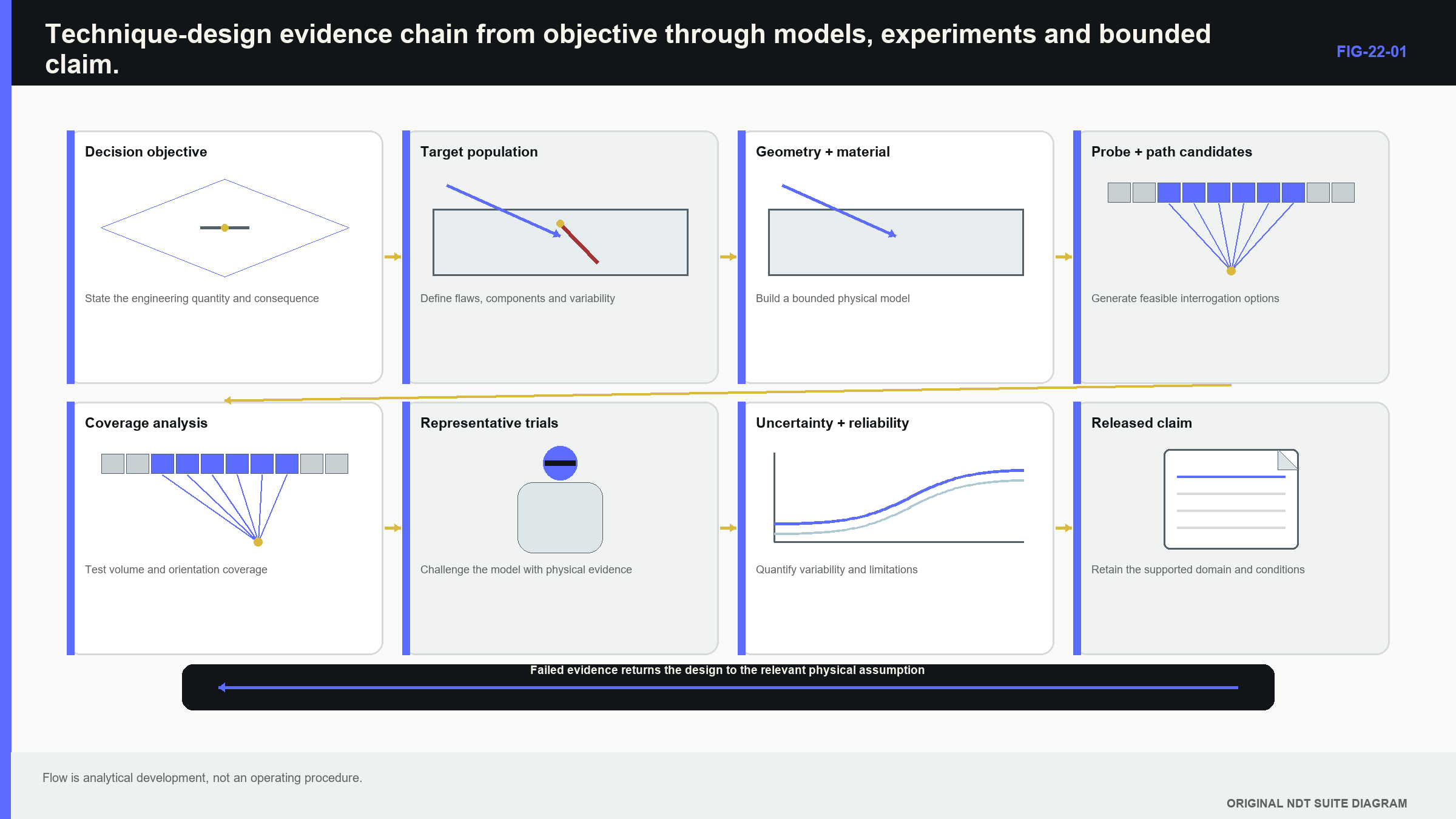
The following figure lays out this evidence chain; notice the feedback loops. Failed coverage or representative response returns the design to an earlier choice instead of being explained away after release.
22.5 Select frequency, mode and aperture
The candidate field must interact with the target and survive the path; frequency balances wavelength, pulse length, scattering, attenuation and resolution. Mode influences target traction, interface transmission and material loss. Aperture changes sensitivity, beam width, focus and tolerance to position. The running case can begin with two shear-wave frequency candidates because fine-grained ferritic material and a fusion-oriented planar target make that a plausible baseline. The comparison should use measurable outputs: target signal-to-noise, separation from root or attachment geometry, field width, coordinate consistency and stability across expected surfaces.
| Worked example · Choosing between two candidate frequencies WE-22-02 Given: On representative coarse material used as a conservative challenge, 5 MHz gives a -6 dB lateral width of 3 mm and target signal-to-noise ratio (SNR) of 4 dB. At 2 MHz, width is 7 mm and SNR is 14 dB. Required target separation is 10 mm, and detection is the primary objective. Find: The better-supported starting frequency. Steps: Both measured widths are below the required 10 mm separation. The 2 MHz candidate has 10 dB greater SNR. Compare the objective rather than selecting the smallest beam automatically. Answer: The 2 MHz candidate has the stronger starting case for detection under the stated conditions. Technical implication: Representative testing should confirm that the 7 mm field still separates the target from nearby geometry. Detection margin outweighs unused nominal resolution in this comparison. Common mistake: Selecting 5 MHz solely because its beam is narrower ignores its marginal target response. |
|---|
This result does not make 2 MHz universally better; a longer low-frequency pulse can reduce axial separation. A larger aperture may improve directivity and sensitivity while increasing footprint and access difficulty. Candidate selection should expose trade-offs that later evidence can test.
22.6 Turn access into a coverage model
Coverage is a spatial and orientation argument; the geometry model should show the target zone, beam envelopes, scan positions, increments, inaccessible regions and relevant target normals. A centreline reaching the target does not prove that useful field covers it. An area percentage does not prove the incidence direction can return a target response. Detection and sizing coverage are different; detection may be supported where one stable target interaction exists. Height sizing can require two identifiable extremities from one or more paths. The running case releases detection and location first, so its coverage model should not silently claim sizing.
Coverage margin is the overlap or response retained after expected variation is included; angle, index, component position, velocity, surface shape and field width can all consume margin. A nominal beam centre exactly touching the edge of the target zone has no robust margin.
| Worked example · Estimating robust overlap under positioning uncertainty WE-22-03 Given: The narrowest measured -6 dB beam width in the target zone is 8.0 mm. Nominal scan increment is 5.0 mm. Lateral probe-position uncertainty is +/-0.8 mm for either adjacent pass. Find: Nominal overlap and conservative remaining overlap when neighbouring passes shift apart by the stated bounds. Steps: Nominal overlap is 8.0 - 5.0 = 3.0 mm. Opposite position shifts consume 0.8 + 0.8 = 1.6 mm. Remaining overlap is 3.0 - 1.6 = 1.4 mm. Answer: Nominal overlap is 3.0 mm, and bounded remaining overlap is 1.4 mm under this position model. Technical implication: Position uncertainty materially consumes coverage margin even when nominal increment is less than beam width. Common mistake: Using a beam width measured in water or at another depth without transfer evidence can make the overlap calculation precise and irrelevant. |
|---|
Orientation margin is separate; a broad sector or several probe angles can improve angular access, but their sensitivity and aperture behaviour may differ. The coverage record should distinguish geometric path access, useful field strength and plausible target interaction.
22.7 Identify essential variables through sensitivity
The candidate technique now has enough structure to identify essential variables; each variable needs a causal route to an objective. Frequency affects penetration and resolution. Wedge condition affects delay, index and angle. Scan increment affects spatial gaps. Filter changes can affect pulse separation and timing. Surface state affects coupling. Operator access affects actual scan positions. A sensitivity study perturbs inputs and observes a relevant output; for small smooth changes, a first-order model is useful.
| (22.1) First-order output sensitivity · EQ-22-01 Where: y = model output; g = measurement model; x_i = influential inputs; Delta = small perturbation Model limits: locally differentiable model and sufficiently small perturbations; interactions require higher-order treatment |
|---|
This relationship supports ranking near one operating point; it does not prove behaviour across mode changes, clipping or thresholds. Level 3 can use supplied derivatives or simple geometry to estimate which variable needs stronger control. Full Jacobian derivation is in Chapter 64.12.
| Worked example · Ranking essential variables for a depth claim WE-22-01 Given: Depth is calculated as z = S cos(theta). Expected ranges are S = 80 +/- 0.5 mm and theta = 60 +/- 1 degree. Find: Approximate first-order depth change from each variable near nominal. Steps: Path sensitivity is cos60 = 0.5, giving 0.5 x 0.5 = 0.25 mm. Angle sensitivity magnitude is S sin60 = 69.3 mm/rad. One degree is 0.01745 rad, giving 69.3 x 0.01745 = 1.21 mm. Answer: Angle range contributes about 1.21 mm compared with 0.25 mm from path range, nearly five times larger in this depth model. Technical implication: Refracted-angle evidence deserves stronger control for this claim. A surface-coordinate output could rank the variables differently. Common mistake: Treating degrees as radians in the sensitivity calculation creates a large numerical error. |
|---|
The ranking guides design; it does not allow low-ranked variables to be forgotten. A variable with little local effect can become important at a threshold or in combination with another variable.
22.8 Design for robustness rather than one perfect setup
Robustness means acceptable performance across the intended variable range; the sharpest focus or largest peak at nominal conditions is not automatically the best design. A narrow focus can lose a target when velocity or probe position changes. A broader field may deliver lower peak amplitude but stronger minimum coverage. For the running case, robustness trials should include thickness extremes, both surfaces, plausible angle and index shifts, representative coupling, more than one operator and target orientations near the envelope boundary; the measured output must match the claim. Detection trials need calls and false calls. Location trials need coordinate error. Sizing trials would need bias, spread and failures to size.
The technique documentation should preserve the reasoning as well as settings; it identifies component and coordinate system, probe and wedge, modes, scan positions, sensitivity basis, acquisition and processing, expected evidence and limitations. A settings list without the physical reason is difficult to review or adapt. Routine controls also arise here; reference response, wedge delay and index, acquisition completeness and software identity are selected because they indicate whether the deployed system remains connected to the design evidence. They are not miniature qualifications.
22.9 Design representative physical evidence
A representative specimen includes the material, geometry, surface, target path and response features that matter to the objective; one block rarely serves calibration, qualification and blind performance equally well. Calibration artefacts establish measurement references; development specimens support access, field and parameter choices. Qualification specimens challenge performance across the intended domain. Blind specimens reveal combined system and human behaviour without expectation from target location.
Truth and realism can conflict; machined notches offer clear dimensions and stable placement but simplified morphology. Natural fatigue cracks give more realistic interaction but require destructive sectioning or complementary characterisation for truth. Truth uncertainty belongs in sizing comparison. An apparent 0.5 mm ultrasonic bias is not established when the target height is known only within +/-0.8 mm. Specimen layout can also create dependence; nearby targets can shadow or interact. Repeated scans of one target estimate repeatability but do not create material diversity. The evidence programme should state what each specimen contributes instead of treating raw scan count as independent support.
22.10 Verify the model and validate its use
Verification checks implementation; for a calculation or simulation, it can include analytical benchmarks, mesh and time-step studies, conservation checks and code tests. Validation compares model output with physical evidence for a stated use. A simulation can be verified and still use the wrong geometry, boundary or material; a travel-time match can validate timing while leaving amplitude unvalidated. A beam-profile match in homogeneous plate does not validate scattering through a coarse repair zone.
The applicability domain names the geometry, material, frequency, modes, targets and outputs covered by the comparisons; extrapolation outside that domain should be visible. Computational NDE can explore difficult systems and variables [R038], but visual complexity is not evidence of applicability. Model discrepancy is the remaining model-to-reality difference after input uncertainty is considered; it can be carried as additional uncertainty, a correction with uncertainty, or a limit on use. Tuning uncertain inputs until one plot matches can hide discrepancy. Independent validation cases are stronger than reuse of the same development data.
22.11 Add interactions only after the basic case is stable
One-variable-at-a-time trials show local trends but can miss interactions; frequency may have little effect in fine-grained parent material and a large effect in coarse repair material. Angle error may be harmless in a broad field and serious near a tight focus. Surface roughness may matter mainly at higher frequency. Designed experiments distribute combinations efficiently; randomisation prevents drift or operator learning from being confused with a candidate technique. Blocking groups known factors such as material batch or day. Replication estimates variation. These ideas support the physical experiment; they do not replace it with statistics.
Full factorial, space-filling, Monte Carlo and robust-optimisation methods belong after the learner understands the physical variables and outputs. Chapter 64.10 provides optimisation foundations. Chapter 70 covers simulation and validation. Chapters 78.3, 78.5 and 78.18 develop uncertainty propagation, designed measurement studies and information-based planning.
22.12 Technical decision case and bounded release claim
The running case can now be closed without overstating it; suppose representative trials show stable detection and location for planar fusion-face targets over the stated ferritic thickness, surface and orientation ranges from two-sided access. The field and overlap evidence provide margin. Location uncertainty remains inside the project need. Height sizing is inconsistent when upper-tip response is obscured. The supported claim can state detection and location for that population and configuration; it can state that crack-like classification uses declared multi-view evidence. It should mark height as informational or outside the released claim. Any coarse-grained repair zone or inaccessible surface lies outside the demonstrated domain unless separately tested.
This bounded statement is stronger than “the weld is covered.” It identifies what the system can establish, the variables that maintain validity, the evidence used and the regions needing another method or design. A limitation is not a failed design when it is detected and communicated before the decision depends on it. The final design record forms a traceable tree:
engineering need -> objective -> target population -> physical models -> candidate technique -> coverage and margin -> essential-variable ranges -> representative evidence -> uncertainty and reliability -> released claim Each branch can be reviewed backward for support and forward for change impact.
In plain words
- Technique design begins with the decision and credible target, not available equipment.
- Detection, location, characterisation and sizing objectives must remain separate.
- Target population includes morphology, orientation, position and surrounding material, not size alone.
- Ray, field, specimen and blind evidence answer different design questions.
- Coverage needs spatial, orientation and uncertainty margins.
- Essential variables are identified through their effect on a stated output.
- Verification checks implementation; validation checks adequacy for intended use.
- A useful release claim states both demonstrated capability and exclusions.
Key terms
- Objective: measurable output required from the technique.
- Damage-mechanism envelope: plausible range of targets from one mechanism.
- Coverage margin: coverage remaining after expected variation.
- Robustness: acceptable performance across intended conditions.
- Sensitivity study: change in output caused by changed input.
- Interaction: dependence of one variable’s effect on another.
- Verification: evidence that a model was solved or implemented correctly.
- Validation: evidence that the model is adequate for a declared use.
- Applicability domain: supported boundary of model or technique use.
Key relationships
- Delta_y approximately sum((partial g/partial x_i) Delta_x_i): first-order sensitivity ranks small local influences.
- coverage margin = nominal overlap - variation consumed: robust coverage is smaller than nominal coverage.
- objective -> evidence -> bounded claim: each claim must trace to representative support.
Common mix-ups
- The smallest target is not automatically the least detectable target.
- A ray reaching a point does not prove useful field or target response.
- Verification is not validation.
- A qualification specimen is not automatically a calibration artefact.
- Optimising peak response is not the same as optimising robust performance.
Bridge to Chapter 23
Chapter 22 ends with representative detections and a bounded claim; chapter 23 examines how repeated outcomes support a population reliability statement. It starts with the familiar result of 19 detections in 20 trials and separates observed fraction, estimated probability and confidence.
Sources and further study
- [R038]
- [R041]
Study and revision only. This is not an approved inspection procedure, acceptance criterion or qualification.