Acquiring FMC Without Losing the Evidence

Why this matters

TFM and PCI can be recalculated many ways, but only from information that survived acquisition; a wrong colour scale can be changed later. A different justified velocity can be tested later. Clipped RF shape, an omitted time window, unstable coupling and missing encoder positions are different; the original evidence has been damaged or never recorded. This chapter follows one matrix from firing to storage, then uses five common failures to decide whether reprocessing remains possible or whether the component must be scanned again.

What you already need

• The Chapter 47 picture of matrix rows, columns, cells and time samples.
• Basic PAUT gain, range, filters, element checks and encoder controls.
• The difference between raw RF, an envelope and a displayed image.
• Familiarity with clipping, noise and loss of coupling.
• Confidence multiplying counts and converting bits to bytes.

What you will learn

• Describe one complete FMC acquisition cycle at one physical position.
• Distinguish full, half and reduced matrix records.
• Recognise clipping, missing channels, poor coupling, short range and position error.
• Select time, sampling and gain controls for usable stored waveforms.
• Estimate the uncompressed data payload for a scan.
• Decide whether a fault permits controlled reprocessing or requires reacquisition.

Words you will meet

• Matrix cycle: the complete declared set of transmit events and receive records at one position.
• Clipping: loss of waveform shape when the signal exceeds the receiver or digitiser range.
• Time origin: the stored reference that connects sample time to physical travel time.
• Matrix scheme: the declared transmitter-receiver pair population that is acquired.
• Dropout: a missing trace, matrix or encoded position.
• Recoverability: whether retained information still supports a valid corrected result.
• Payload: the stored sample bytes before file overhead and supporting records.

48.1 Follow one matrix cycle

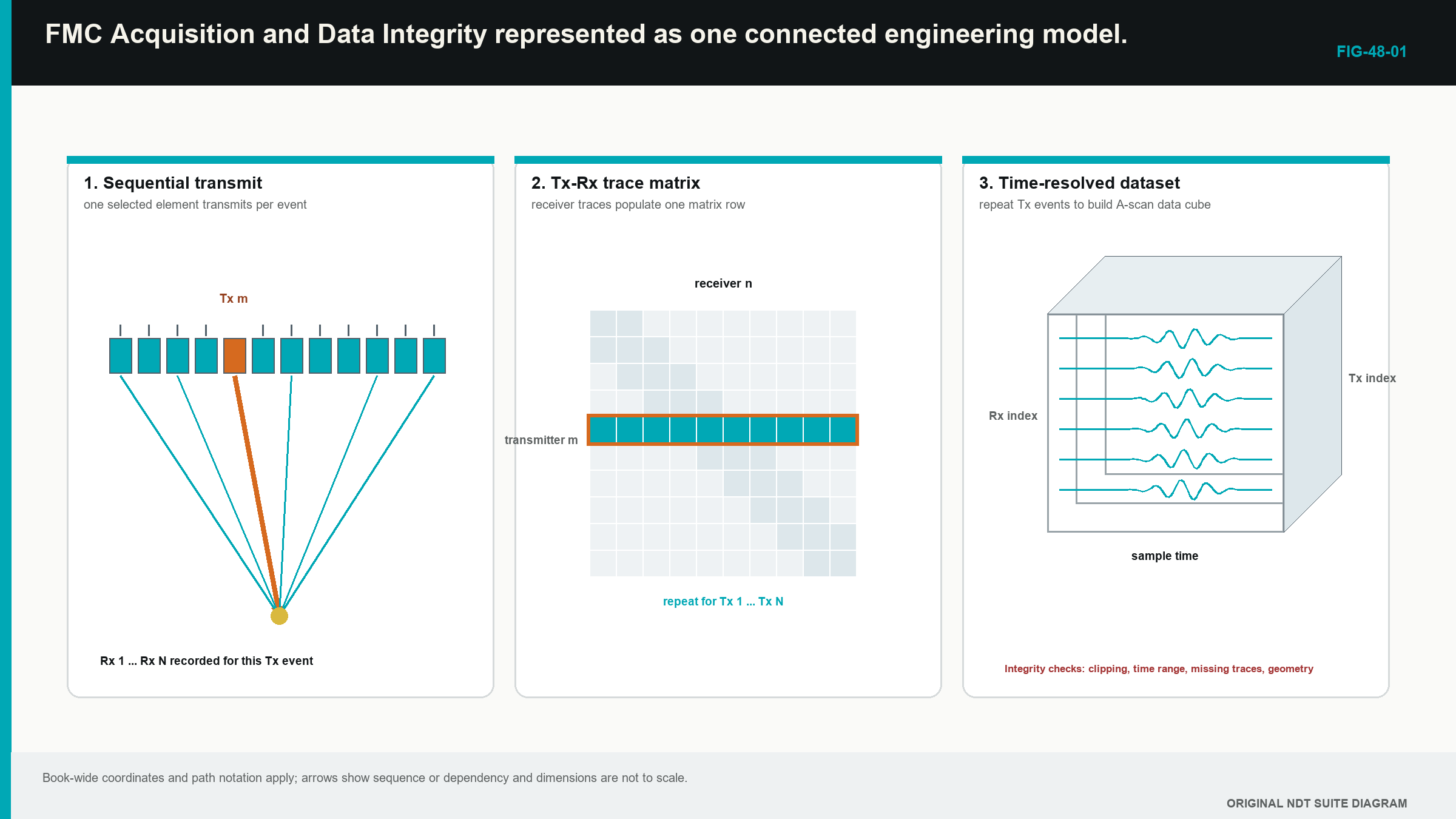
At one stationary probe position, the instrument selects the first transmitter and fires it; the declared receivers record their A-scans over the selected time range. The instrument stores those traces with transmitter and receiver identities; it then selects the next transmitter and repeats the event until the required pair population is complete.

Only after that complete cycle represents one position should the scan advance to the next encoded location. Hardware may record several receivers in parallel or route them through multiplexers, but the Level 2 control remains the same. The technician must know which pairs belong to one position and whether the instrument completed them before motion changed the acoustic state.

The following figure shows the record growing from one row into a time-resolved matrix and then along the scan. Notice that position is attached to the complete matrix, not guessed from the final image.

The actual acquisition architecture belongs in the record. A TFM screen can be produced from full FMC, a reduced matrix, a plane-wave sequence or another documented source. Reconstruction software does not retroactively make those sources identical. Published and training material on matrix acquisition emphasises retained pair identity, adequate sampled signals and controlled position information as prerequisites for later reconstruction. [R017] [R023] [R047] [R053]

48.2 Learn the full matrix before meeting reductions

A full matrix records every declared ordered combination of the selected transmitters and receivers; with the same 64 elements in both roles, the nominal population contains 4,096 ordered traces. This arrangement retains the greatest pairwise flexibility of the common sequences introduced here, at the cost of acquisition time, storage and processing.

A half matrix retains one triangular half plus its treatment of the diagonal. It relies on a demonstrated basis for reciprocal reduction. The missing ordered direction may remove diagnostic or performance information when transmit and receive chains differ, conditions change during the sequence or a later algorithm needs both directions.

A sparse or reduced matrix retains selected transmitters, receivers or individual pairs. The selection can speed acquisition and reduce files. It also changes effective aperture, spatial sampling, lobe behaviour and the source information available for another reconstruction. A good result for one target does not establish equivalence for every location and orientation.

Plane-wave and virtual-source families use multi-element transmit events rather than the one-element-at-a-time foundation. They may feed TFM-like or coherence processing, but they remain separate architectures. Chapter 55 compares their information and validation demands at Level 3. At this stage, the learner reads the acquisition label and does not assume that all advanced images started as full FMC.

48.3 Five losses that look different in the final image

Clipping occurs when a waveform exceeds the usable electrical range. Its peaks flatten and the original amplitude, curvature and phase are lost. Lowering display gain afterwards only makes the flattened trace smaller. It cannot restore the missing shape.

A missing channel can appear as a weak row, weak column or absent set of cells. A validated exclusion may allow a demonstrated reconstruction to proceed, but copying a neighbour into the gap invents data. The change in pair population and aperture remains recorded.

Poor coupling reduces or distorts many paths through the affected part of the aperture. If coupling changes during the sequential matrix cycle, the stored pairs no longer represent one consistent acoustic state. A later normalisation can make them similarly bright while hiding that inconsistency.

A wrong or short time range can omit long off-diagonal, skip or mode-converted arrivals. The processor cannot sample beyond the stored record. Extending the region of interest (ROI) later merely produces pixels with incomplete time support.

A wrong encoder position attaches a good matrix to the wrong component coordinate. Reconstructing the local cross-section again does not recreate the missing or misassigned scan location. These five examples establish the main rule: display and model errors may be reprocessed when source data survive; acquisition loss normally requires reacquisition or an authorised limitation.

48.4 Walk through the acquisition signal chain

The pulser sends an electrical drive to the selected element. Pulse voltage, width, damping and firing rate influence transmitted energy and spectrum. Too much drive can produce receiver recovery problems or clipping. Too little can leave long paths near noise.

The element, matching layers, wedge or couplant and component interfaces shape the acoustic pulse. Uneven contact can change delay, bandwidth and amplitude across the aperture. Surface roughness, temperature and probe rocking can make those changes vary with position.

The receiver applies analogue gain and filtering before the digitiser stores samples. Gain must accommodate both strong short paths and weak long paths. Analogue filtering prevents unwanted content reaching the sampler, but content removed at that point is unavailable to every later reconstruction.

The digitiser converts the voltage to values at fixed time intervals and within a finite numeric range. Digital filtering, averaging, compression, rectification or sign reduction may occur before storage. Each operation changes what can be recovered later. The controlled configuration therefore records the stored signal form rather than relying on the comforting but vague word raw.

48.5 Give every required path enough time

Start with the longest justified transmitter-to-interaction-to-receiver route. Include wedge legs, component legs, backwall reflections, conversions and the farthest relevant reference target. Add a stated margin for geometry and velocity variation. The selected record also needs a clear time origin so stored sample number can be related to physical travel time.

An electronic delay, a wedge transit time and a component zero are not interchangeable. If the acquisition origin is 2 microseconds before the wedge entry event, the reconstruction model must know that offset. Silently adjusting image depth until one target aligns can conceal the wrong time model and misplace other regions.

Sampling rate controls the time spacing between stored values. It must represent the retained signal band closely enough for location and phase-sensitive processing. A higher rate creates more samples and larger files. It does not add acoustic bandwidth that the probe, material or analogue filters removed. Chapter 58 treats fractional delays and numerical interpolation more deeply.

48.6 Set gain for waveform integrity

Three source-signal zones are useful. Below the usable signal-to-noise region, random voltage can dominate timing and phase. Inside the linear digitiser range, waveform shape and relative timing remain available. Above the range, clipping destroys shape.

Amplitude-free PCI still depends on this source waveform. Removing amplitude from the final metric does not create stable phase in a noise-dominated trace. It also does not reverse saturation. Check representative strong diagonal and near-surface pairs together with weak, wide and long-path pairs. One gain may be unable to make every group useful without clipping; that is a probe, pulser, receiver or technique-design problem rather than a palette problem.

Normalisation belongs after acquisition. It can display weak and strong traces on comparable screen ranges for review, but it must not be mistaken for equal source quality. Retain fixed-scale comparisons and the clipping state.

48.7 Keep coupling stable through the cycle

FMC is sequential. If the probe moves significantly while transmitters fire in turn, early rows and late rows represent different physical locations. If coupling changes during the cycle, reciprocal pairs may differ because they were captured under different contact conditions. Both effects can blur amplitude TFM and create unusual phase behaviour.

The approved technique links scan speed to complete matrix rate and encoded increment. A hand scan that races ahead of acquisition can generate repeated, skipped or position-averaged records. A mechanised scanner can do the same when triggers arrive faster than the instrument can store complete matrices.

Contact should be stable over the whole wedge or probe face. Surface scale, weld spatter, curvature and temperature can disturb one side of the aperture more than the other. A dedicated coupling signal, backwall channel or other approved indicator remains important when phase processing suppresses broad interface responses.

When contact is lost, the defensible action is to stop at a traceable position, restore the cause and repeat the affected region with the required overlap. Continuing with the hope that reconstruction will repair contact later is optimism wearing safety boots.

48.8 Protect encoder and scan-position integrity

Before scanning, verify encoder distance, direction sign, index offset and origin against an independent physical reference. During the scan, watch for wheel slip, lift, backlash, reversal, repeated positions, missing triggers and discontinuities. After the scan, compare stored start and end locations with physical marks and the required extent.

A fine image grid does not compensate for coarse encoded sampling. Reconstruction-grid spacing controls calculated points inside one frame. Encoder increment controls where complete acoustic frames were actually collected along the component. Mixing those two axes can produce very precise-looking gaps.

The position record should contain the expected count, monotonic direction where appropriate and controlled handling of repeated or interrupted segments. If the file joins scans, each segment and overlap remains identifiable. A complete matrix attached to the wrong weld, side or datum is not useful evidence merely because every checksum passes.

48.9 Estimate data before the instrument fills up

One trace contains a selected sample count and stored bits per sample. Multiply by pair count for one frame and by encoded positions for the scan. Divide bits by eight to obtain bytes.

The equation estimates sample payload only. File containers, position tables, setup records and integrity information add overhead. Compression can reduce stored size while changing access or recoverability, so it belongs in the declared architecture.

48.10 Preserve the configuration with the data

The acquisition record links component and examination identity; probe, wedge, cable and instrument; software and firmware version; element map and matrix scheme; pulser and receiver settings; sample rate, filters and time origin; encoder scale, direction and increment; material and geometry information; operator, temperature and coupling notes; setup revision; and pre-use and post-use results.

The preserved original is kept separate from derived reconstructions. A conversion for another software package records the tool, version, input identity and any lost fields. File count, size and an approved integrity check are verified after transfer. A screenshot can support a report but cannot replace pair data when the technique requires later reproduction.

Pair exclusions, smoothing and corrected metadata are never hidden in the original. A working copy can be used for a controlled investigation. The disposition states why the change was made and whether the result remains reportable.

48.11 Decide between reprocessing and reacquisition

A corrected, authorised velocity or component geometry can often be applied to retained data. A different justified path or region can be reconstructed if the required pair traces and time support exist. Display colour, annotations and fixed-scale presentation can be changed. Validated weighting or pair exclusion can be studied on a controlled copy.

Reprocessing cannot create unrecorded time, replace a missing physical scan strip, undo clipping, restore bandwidth filtered out before storage, stabilise coupling that changed during the matrix, or recover a position that the encoder never captured. Missing channels may be usable only when the controlled reduced aperture has demonstrated the intended task.

A completed disposition case starts by classifying the fault as missing data, distorted data, wrong metadata or a derived-display error. It then connects that class to the required detection, location or sizing claim. A colour-map error with intact linear pixels is reversible. A wrong stored time-origin label may be correctable when independent evidence establishes the true offset. A clipped target packet is distorted source data and normally triggers reacquisition.

The Level 3 treatment formalises recoverability through expected and observed pair counts, saturation fraction, channel distributions, reciprocal residuals, position continuity and protected file identity. These measures establish internal dataset condition; they do not by themselves prove application performance. [R017] [R047]

48.12 A controlled acquisition narrative

Before scanning a weld-like specimen, the operator confirms the released setup, physical extent and target paths. The matrix scheme, time origin, sampling, stored RF type and predicted payload are recorded. Channel, timing, clipping and encoder checks pass on the identified reference specimen. Available storage exceeds the estimate with margin.

During the scan, the operator maintains full contact below the demonstrated speed and watches raw range, position and dropped-data indicators. A short coupling interruption appears at 186 mm. The scan stops, the cause is corrected and the affected section is repeated from 180 mm with controlled overlap. The original interrupted segment remains identified rather than silently deleted.

Post-use checks pass. Stored position count and physical marks agree. The raw source, setup and auxiliary records are transferred and integrity-checked. The final disposition accepts the repeated segment and marks the interrupted segment non-reportable. No reconstruction was used to disguise the acquisition event.

This narrative contains the field workflow without turning the teaching chapter into an operating instruction. The approved organisational procedure remains the source of actual tolerances, hold points and record forms.

Step up

Chapter 55 develops full, half, sparse and plane-wave architectures as Level 3 design choices. Chapter 58 treats numerical reconstruction and fractional delay. Chapter 62 develops forensic tests for acquisition faults, while Chapter 80 treats throughput, storage and system architecture. The Level 2 boundary is to recognise what survived, what was lost and when the defined technique requires a new scan.

In plain words

• One FMC matrix cycle must represent one controlled acoustic state at one position.
• Full, half and sparse matrices retain different pair information.
• Clipping destroys waveform shape; reducing display gain later does not restore it.
• The time range must include every required direct, reflected or converted arrival.
• PCI still needs usable, unclipped source signals even when amplitude is absent from the final scale.
• Matrix rate, scan speed and encoder increment must allow complete positioned records.
• Data payload should be estimated before scanning and stored with its configuration.
• Reprocessing fixes supported model or display choices, not missing acquisition evidence.

Key terms

• Matrix cycle: all declared pair events attached to one accepted position.
• Clipping: irreversible loss of waveform shape beyond the acquisition range.
• Time origin: reference connecting stored sample time to the travel-time model.
• Matrix scheme: full or reduced pair population actually retained.
• Dropout: missing source trace, frame or position.
• Recoverability: valid correction possible from surviving source information.
• Payload: sample bytes before additional file overhead.

Key relationships

• matrix cycle + encoded position: a reconstruction frame needs both pair data and a physical location.
• B_frame = N_pair N_s b / 8: pair count, samples and stored bit depth determine sample bytes at one position.
• B_dataset = N_pos B_frame: accepted positions multiply the frame payload.
• source loss -> reacquisition: information never recorded or destroyed before storage cannot be restored by image processing.

Common mix-ups

• A TFM screen does not reveal whether its source was full FMC or a reduced architecture.
• Digital normalisation is not recovery from low signal or clipping.
• Reconstruction pixel spacing is not encoded scan increment.
• A missing pair and an authorised reduced pair population are not the same condition.
• A successful file transfer does not prove that the acquisition itself was valid.

Bridge to Chapter 49

Chapter 48 has secured the source information. Chapter 49 now uses that information to build one TFM pixel. It begins with one point and two travel legs, then repeats the same calculation across the image region.

Sources and further study

• [R017]
• [R023]
• [R047]
• [R053]