
CHAPTER 17 · Ultrasonics Level 2
Size Only What the Signal Can Support
In this chapter · 21 sections
Why this matters
An echo remains visible for 18 mm along a weld, while two small signals appear 6 mm apart in depth. Those are different measurements. The first may mostly describe response extent and beam width; the second may be an estimate of reflector height if the signals are genuine tips. Sizing becomes unsafe when a display dimension is quietly renamed as a physical flaw dimension. This chapter starts with the feature on the screen, matches it to a suitable method and adds a practical statement of uncertainty. The more formal mathematics is deliberately left for Level 3 and the engineering Part.
What you already need
- Reliable detection, location and response characterisation.
- Basic dB comparison and angle-beam plotting.
- The ideas of beam width, pulse length and spatial sampling.
- How to distinguish a face response from possible tip or edge responses.
What you will learn
- How to name the dimension before selecting a sizing method.
- What amplitude-drop, tip-time, geometric and equivalent-reflector methods measure.
- How corrosion mapping differs from weld-flaw sizing.
- How to describe repeatability, bias and uncertainty in practical language.
- How to report an estimate, limit or unresolved result honestly.
Words you will meet
- Response extent: the region over which an echo meets a stated display rule.
- Extremity: an end, edge or tip used to estimate a reflector boundary.
- Equivalent reflector: an ideal reference target giving a comparable response under a stated model.
- Bias: a repeatable tendency for a method to read high or low.
- Repeatability: variation when a measurement is repeated under closely controlled conditions.
- Uncertainty: the reasonable spread around a measurement result under its stated model.
- Ligament: remaining distance from a reflector extremity to a component surface.
17.1 Name the dimension before measuring it
Write a plain statement of the required quantity. Examples are minimum remaining wall, reflector depth, projected response length, estimated planar height, ligament to the surface or equivalent reflector size. The formal name for the intended quantity is the measurand, but the plain statement matters more than the label.
Do not treat these dimensions as interchangeable. Response length includes reflector behaviour, beam footprint, scan direction, threshold and processing. Tip separation depends on correct extremity identification and location. An equivalent-reflector result compares amplitude with an ideal target; it is not automatically a crack diameter. A corrosion thickness comes from locating a boundary, not from measuring flaw-echo amplitude.
The sizing method must answer the dimension the engineering decision actually uses. If the assessment needs through-wall height, a long above-threshold response along the weld does not supply it.
The following figure separates the common dimensions and shows which input can influence each one.
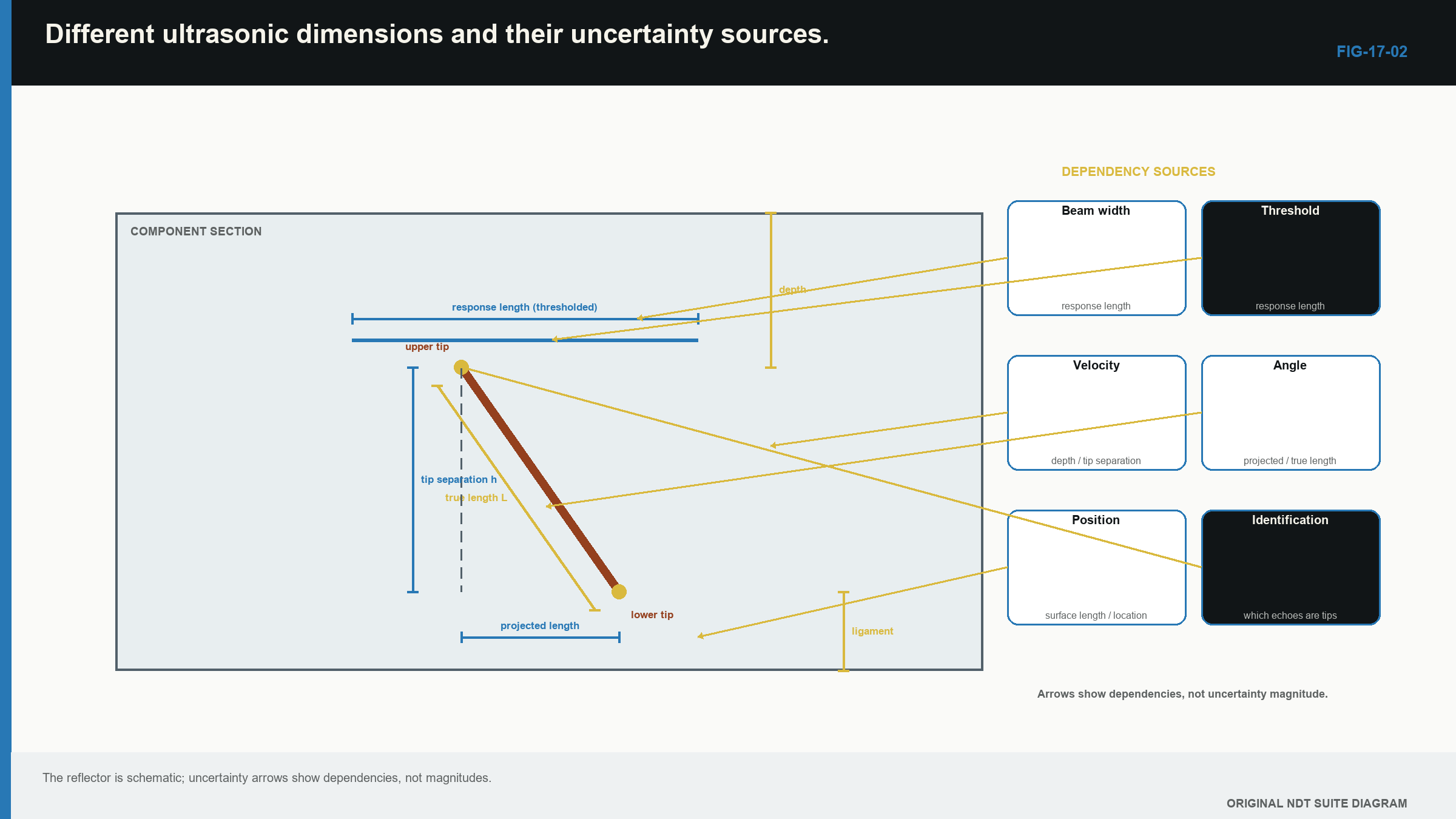
Notice that response length, depth, height and ligament are different results with different uncertainty sources.
17.2 Start with the observable feature
Before choosing a method, describe what the data actually contain. Record whether there is one unsaturated face echo, whether two distinct extremity signals are resolved and whether the back wall remains trackable across a corroded surface. Also record whether an encoder is available and whether a representative target behaves in the same way.
If the required feature is absent, do not force the method. A saturated face cannot support a meaningful amplitude drop. One unresolved broad pulse cannot reliably become two tips. A lost back wall cannot be converted into a precise thickness simply by moving a cursor to the last noise peak.
A bound may be the correct result. An upper extremity may be visible while the lower one merges with the back wall, supporting a ligament or minimum-height statement rather than a full height. A target smaller than demonstrated resolution may be reported as unresolved below that capability, not as zero.
17.3 Amplitude-drop sizing
An amplitude-drop method begins at a peak response and finds positions where the signal falls by a stated number of decibels. The distance between those positions is then converted into a response dimension. Under comparable voltage-amplitude conditions, a 6 dB fall is about half the peak amplitude, while a 20 dB fall is about one tenth.
The drop value is a measurement rule, not a universal accuracy guarantee. For a small reflector moved through a smooth beam, the width between drop points may mainly describe the beam. For a larger planar face, it may better follow where the beam crosses reflector edges. Orientation, roughness, saturation and threshold stability change the answer.
Keep the setup controlled and record the rule, direction and endpoints. If a representative study shows a stable bias for the same beam, target family and analysis, a justified correction may be applied. Do not transfer the correction to another angle, frequency, reflector orientation or processing method without evidence.
| Worked example · Separate response length from estimated reflector length WE-17-02 Given: A directional weld response remains above a 6 dB drop rule for 18.0 mm along the weld. A representative study using the same scan geometry found that this method reads known planar reflectors 3.0 mm long on average, with result scatter represented by 1.5 mm. Positioning contributes another 0.8 mm of uncertainty. Treat the two uncertainty contributions as unrelated for this simple example. Find: The corrected length estimate and the combined practical uncertainty scale. Steps: Correct the demonstrated average bias: 18.0 mm - 3.0 mm = 15.0 mm. Combine the two unrelated contributions by root-sum-square: sqrt(1.5^2 + 0.8^2) = 1.70 mm. Answer: The estimated length is 15.0 mm with a combined standard uncertainty scale of about 1.7 mm, before other model limits are added. What it means in practice: The observed 18.0 mm is response length. Converting it into estimated reflector length depends on representative performance evidence. Common mistake: Applying the 3.0 mm correction to a different probe, angle, threshold or reflector family. |
|---|
17.4 Tip and time-based sizing
Edges and crack tips can diffract sound. When upper and lower extremity responses are separately identified and correctly located, their coordinate separation can estimate through-wall height. This can reduce dependence on specular face amplitude, but it does not remove path, velocity, timing or identification uncertainty.
Tip responses may be weak. A facet, root corner or mode-converted path can imitate one. Beam width and pulse length may merge two nearby tips. Change angle or access to test the positions, and keep the face echo unsaturated so it does not bury the extremities.
Record which signals were called as tips and which views support them. If repeated analysts select different peaks, that spread is part of practical performance. “No second tip resolved” is an observation; it is not evidence of zero height.
17.5 Geometric and equivalent-reflector methods
Geometric sizing uses known boundaries, shadows, intersecting paths or probe coordinates. Its quality depends on correct component dimensions and correct association between the signal and the proposed boundary. A shadow may establish that a feature blocks part of a path without uniquely giving its shape.
DGS and related amplitude methods compare a response with the modelled response of an ideal reflector. The output is an equivalent size within that method. It supports consistent comparison but should not be renamed as actual crack diameter or pore diameter.
Choose the method according to the observed response. A strong smooth face may support a demonstrated amplitude rule. Resolved extremities may support tip separation. Stable boundary echoes support thickness or geometry measurement. If none is present, an honest limit is more useful than a precise invented dimension.
17.6 Corrosion mapping measures a boundary
For corrosion, the common quantity is remaining wall thickness. The screen must identify the relevant front and back boundaries, accounting for coating, delay line and any multiple-echo method. Rough or steep pits can reflect energy away. A pit smaller than the beam can be averaged with thicker surrounding wall. Deposits or laminations can create another echo that is mistaken for the back wall.
Use movement and echo pattern to maintain boundary identity. Compare adjacent sound material and, where permitted, another surface or probe. A dense scan grid improves spatial sampling but cannot make the beam footprint smaller. A deep narrow pit can still lie between grid points or be averaged inside a larger beam.
For trending, return to the same coordinates and comparable surface, temperature and setup. A change of datum can look like metal loss. Store observed points separately from interpolated colour maps; the smooth surface drawn between points was not directly measured.
17.7 Plate, weld and corrosion case comparison
The same sizing word can hide different measurements.
In plate, map the region where a lamination response replaces or reduces the back wall. The mapped boundary is influenced by beam footprint and scan spacing. In a weld, a face-response length along the seam may not equal physical flaw length, while two verified tips may support a height estimate. In corrosion, the minimum recorded thickness is a boundary measurement whose reliability depends on beam footprint, pit shape and point spacing.
Before reporting any of these, state the signal feature, the conversion model and the main limitation. This three-part statement prevents a screen measurement from quietly becoming a physical dimension during later engineering assessment.
The following figure shows why several reflector shapes can remain plausible from one limited view.
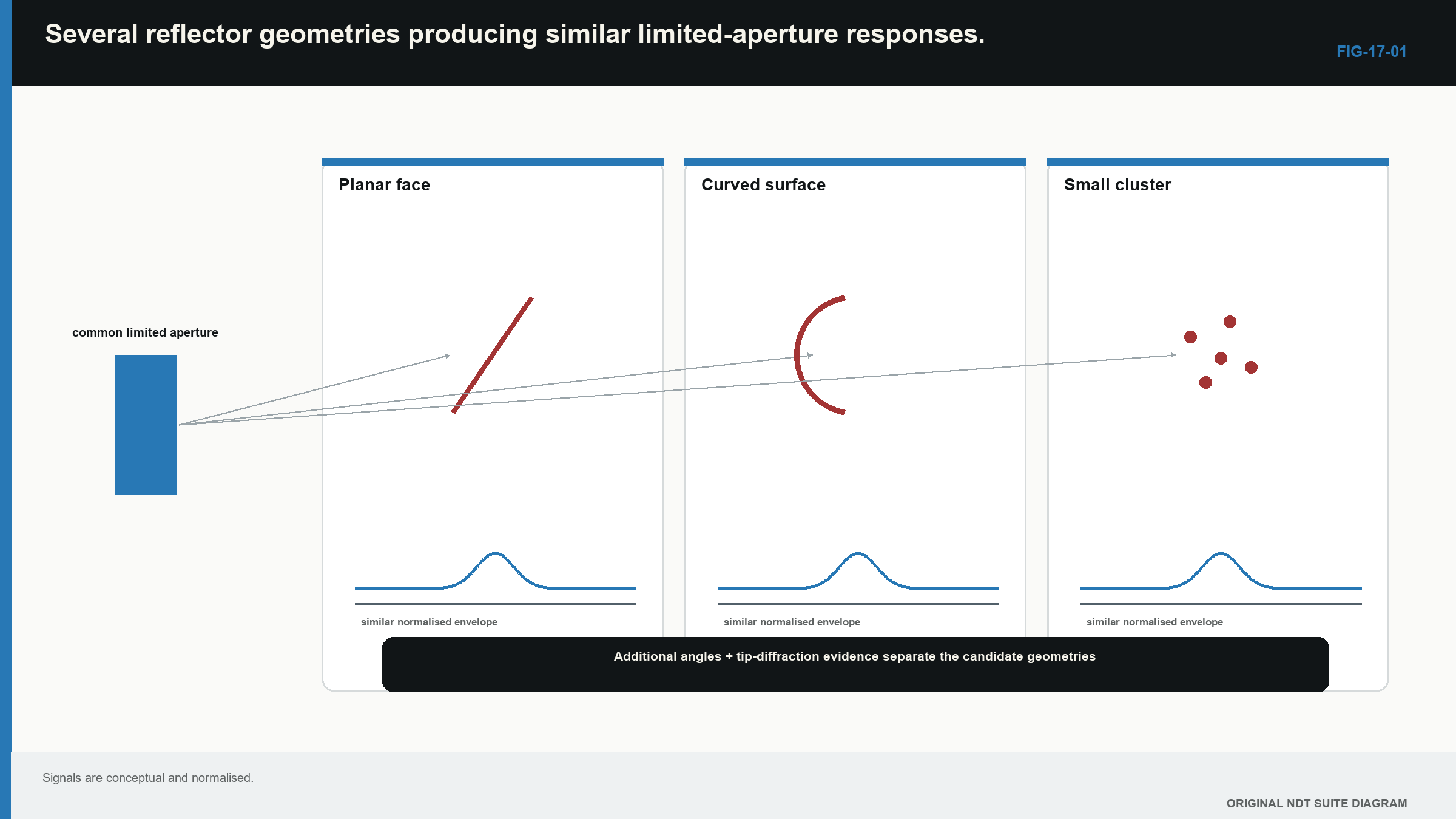
Notice that another angle or reliable extremity signal adds information; it does not make the model disappear.
17.8 Build a practical uncertainty statement
Every result has variation and model limits. Repeat the measurement after lifting and replacing the probe. Where practical, include another operator or probe. Compare with representative known dimensions. Note calibration resolution, velocity range, angle or index variation, encoder positioning and signal-picking differences.
Some influences behave like scatter. Others shift results mainly in one direction. A stable high reading against representative truth is bias. Correct a known bias when the correction is defensible, then retain uncertainty in that correction. A tight cluster of repeated values can still be wrong if every result shares the same incorrect velocity or signal identity.
General uncertainty guidance distinguishes estimates from repeated observations and estimates from other evidence such as calibration, resolution and material bounds. [R031] [R032] Formal sensitivity coefficients, covariance and coverage factors are Level 3 material. EQ-17-01, EQ-17-02, WE-17-01 and WE-17-04 are retained in the migration ledger for that treatment.
At Level 2, report the value, the method, the demonstrated performance range and important unquantified limits. Do not add extra display decimals to make an uncertain method look precise.
17.9 Understand failure to size
Sizing trials often look better when unresolved cases are omitted. If two tips cannot be separated, the method has not produced an ordinary small error around zero; it has reached a resolution limit. If one tip is hidden by geometry, the result may be bounded but not complete.
Track how often the method returns no result and under which conditions. A method that gives accurate dimensions for half the detected targets and cannot size the rest has different field capability from one that returns a moderate-uncertainty result for nearly all targets.
Temperature and environment can also move a method outside its evidence. Temperature changes material and wedge velocity, couplant behaviour, attenuation and probe condition. A room-temperature reference does not automatically support a hot component. Record temperature state and apply only established corrections or limits.
17.10 Put uncertainty beside the decision
The measurement report should not invent an acceptance rule. It should provide the best supported result and the information the governing decision process needs.
When the plausible interval spans a threshold, the measurement alone does not clearly place the quantity on one side. Another suitable measurement, a declared conservative rule or engineering assessment may be required by the governing system. More cursor precision will not fix method-limited uncertainty.
| Worked example · Recognise an unresolved threshold comparison WE-17-03 Given: A measured height is 4.8 mm with stated expanded uncertainty of 1.0 mm. A hypothetical decision threshold supplied for the case is 5.0 mm. Find: Whether the measurement interval lies wholly on one side of the threshold. Steps: The stated interval is 4.8 mm plus or minus 1.0 mm, or 3.8 mm to 5.8 mm. The 5.0 mm threshold lies inside it. Answer: The measurement alone does not resolve which side of the threshold contains the physical height under the stated uncertainty. What it means in practice: Report the result and uncertainty for the governing decision process. Do not turn 4.8 mm into a falsely certain “below 5 mm” statement. Common mistake: Hiding the uncertainty because the displayed central value falls below the threshold. |
|---|
17.11 Report result, method and limit
A useful sizing entry contains:
- the intended physical quantity;
- the observed signal feature and method;
- the result with sensible rounding;
- any demonstrated correction and performance range;
- unresolved identification, coverage or material limits; and
- the coordinates and data identity needed to reproduce the result.
For example: “Projected response length along the weld is 18 mm using the stated 6 dB drop rule. Representative same-setup evidence supports a corrected planar-length estimate of 15 mm with approximately 1.7 mm standard uncertainty before listed material and endpoint limits.” The two dimensions remain visibly different.
The conventional sizing methods and their interpretation limits remain grounded in the international UT training source. [R001] Advanced treatment later in the book will show how formal budgets, correlated effects and engineering decision rules extend this practical foundation.
In plain words
- Name the physical quantity before selecting the sizing method.
- A response dimension is not automatically a discontinuity dimension.
- Amplitude-drop methods depend on beam, target, threshold and orientation.
- Tip separation needs real, resolved and correctly located extremity signals.
- Equivalent-reflector size is a comparison result, not automatic crack size.
- Corrosion mapping measures a boundary and remains limited by beam footprint and scan spacing.
- Repeatability does not remove shared bias.
- An unresolved or bounded result is better than a precise unsupported number.
Key terms
- Measurand: formal term for the quantity intended to be measured.
- Bias correction: supported adjustment for a demonstrated systematic reading difference.
- Censored result: a result known only to be above, below or unresolved within a capability limit.
- Expanded uncertainty: a wider stated uncertainty interval using a declared coverage basis; formal treatment follows later.
- Sizing capability: demonstrated ability of a method across its intended targets and conditions.
Key relationships
- Observed response extent combines target response, beam field, scan path and threshold.
- A corrected estimate equals the observed result minus a demonstrated bias, with correction uncertainty retained.
- Unrelated uncertainty contributions are often combined by root-sum-square; formal conditions follow at Level 3.
- Grid spacing and beam footprint both affect whether a local minimum or endpoint can be captured.
Common mix-ups
- Response length is not automatically flaw length.
- Equivalent-reflector size is not physical crack diameter.
- No resolved tip is not zero height.
- Many repeated measurements do not expose a shared wrong velocity or wrong echo identity.
- A dense colour map does not convert interpolation into measured points.
- Uncertainty cannot rescue the wrong quantity or a misidentified signal.
Bridge to Part III
Part II has built a practical chain from beam and instrument through probe choice, calibration, geometry, materials, interpretation and sizing. Part III keeps that chain but moves into Level 3 responsibility: measurement-system design, qualification evidence, uncertainty models, technical decisions and governance across a defined examination domain.
Sources and further study
- [R001]
- [R031]
- [R032]
Study and revision only. This is not an approved inspection procedure, acceptance criterion or qualification.