
CHAPTER 12 · Ultrasonics Level 2
Calibration, Reference Sensitivity and Reliable Checks
In this chapter · 20 sections
Why this matters
Placing one echo at 80% screen height can look like a complete calibration, but it is not. A reliable setup needs separate evidence for time or distance, probe behaviour, reference amplitude and practical application. Mixing those jobs can hide a wrong scale, wrong angle or unsuitable reference behind a good-looking screen. This chapter follows one setup from known reflectors to a final check and explains both what each comparison proves and what it does not prove.
What you already need
- Range, zero, velocity and delay affect horizontal position.
- Gain affects displayed response height.
- Probe index, angle and beam field can change after wear or substitution.
- Different reflector shapes return sound differently.
- A reference result is useful only under stated conditions.
What you will learn
- Separate time-base, probe, sensitivity and application checks.
- Explain what common reference reflectors are suited to show.
- Read distance-amplitude correction and time-corrected gain correctly.
- Calculate scale, offset and amplitude differences from reference data.
- Explain transfer as a specific comparison, not free extra gain.
- Respond logically when a final check changes.
Words you will meet
- Time-base calibration: connecting echo time to displayed distance.
- Reference sensitivity: setting a controlled amplitude comparison.
- DAC: a distance-amplitude correction curve from known reflectors.
- TCG: time-corrected gain applied across the calibrated range.
- DGS: a model-based distance-gain-size comparison.
- Transfer: a measured difference between reference and component conditions.
- Drift: a change in system response over time.
12.1 Four controls that answer different questions
The word calibration is often used for several activities. Separate them by the question they answer.
Time-base calibration asks whether known path lengths appear at the correct positions. Two separated reference paths help distinguish a constant offset from a scale or velocity error.
Probe-characteristic verification asks whether important probe properties remain correct. For an angle probe, this commonly includes index and actual refracted angle. For a thickness probe, zero and usable range may be central.
Reference sensitivity asks how the complete system responds to a defined reflector. It creates a repeatable amplitude basis.
Application performance evidence asks whether the full technique can reveal the target classes over the required component region. A reference echo can support this evidence, but one convenient target does not prove the entire application.
The stacked figure below shows the dependency. Higher layers need the lower ones, but one layer cannot replace another.
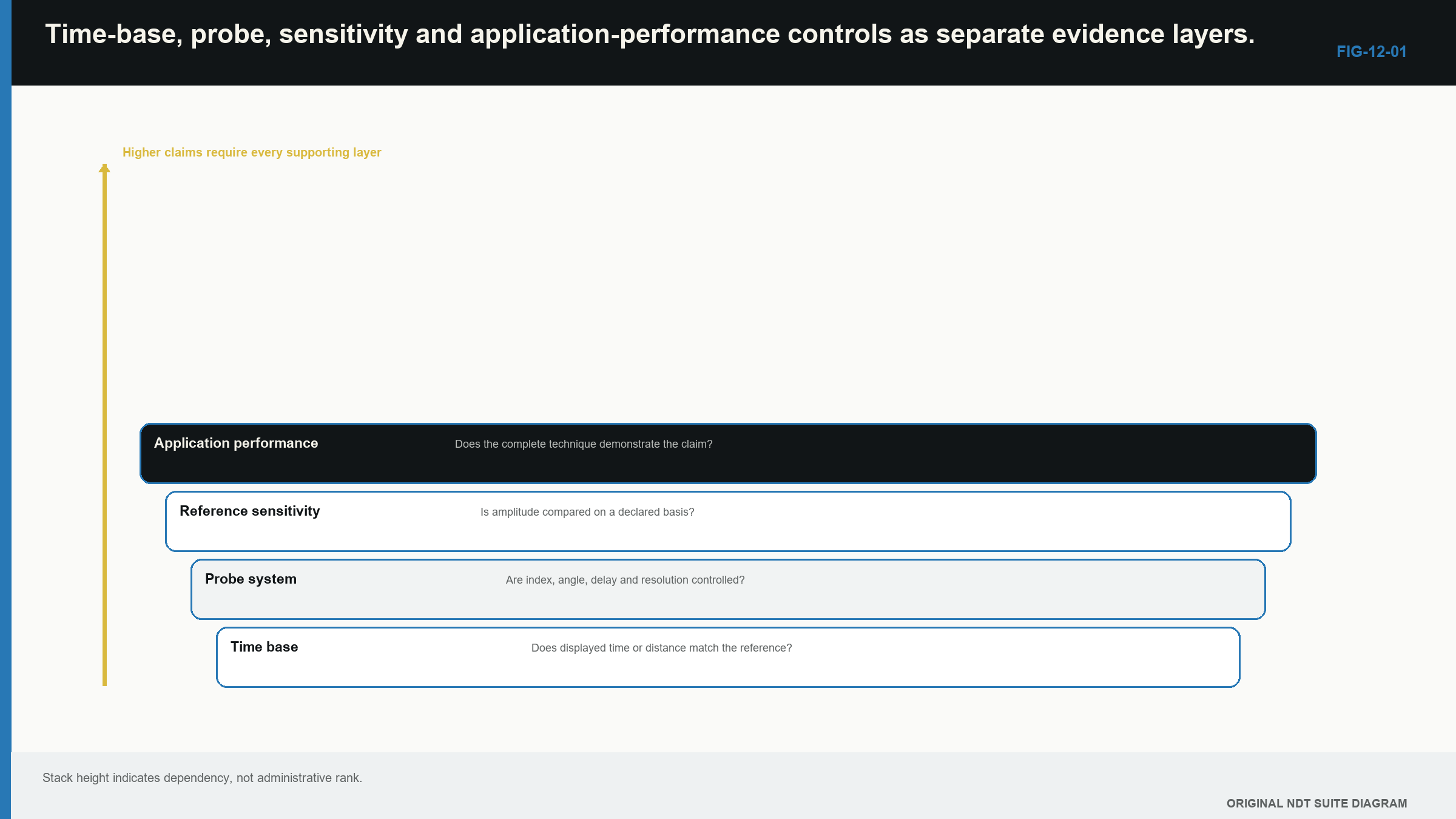
Notice that a higher-layer check needs the lower layers but does not prove every lower-layer property separately.
12.2 Choose the reference for the measurement job
A reference block supplies known material and geometry. The reflector should suit the quantity being checked.
A known radius or thickness can support time-base work, and a radius can also help establish angle-probe index and actual angle. Side-drilled holes provide repeatable responses over several paths, while flat-bottom holes are strongly directional. Notches can provide a surface-connected planar response, whereas back walls are extended specular reflectors.
Equal dimensions do not make these reflectors acoustically equal. Shape, direction and extent change response. A reference hole is a controlled target, not a photograph of a natural crack.
Reference material matters as well. Similar-looking blocks can differ in velocity, attenuation and microstructure. Probe and block behaviour interact, so block identity and measurement purpose belong in the record. [R010]
12.3 Use more than one distance point
One known echo can be placed correctly by changing either zero or scale. A second separated echo shows whether the relationship remains correct across the range.
For a simple linear model, displayed distance is represented by a scale factor and a constant offset.
| (12.1) Linear calibration model · EQ-12-01 Where: d_display = displayed distance; d_true = reference distance in the same units; a = scale factor; b = constant offset Model limits: the time-to-distance relationship is approximately linear over the stated range |
|---|
If a = 1, the scale is correct. If b = 0, there is no constant offset. Two points allow both values to be separated.
| Worked example · Separate a scale error from a zero error WE-12-01 Given: True paths are 50.0 mm and 150.0 mm. The instrument displays 52.5 mm and 157.5 mm. Find: Scale factor a and offset b in d_display = a d_true + b. Steps: Use the change between points for the scale. a = (157.5 - 52.5)/(150.0 - 50.0) = 105.0/100.0 = 1.05 Use either point to find the offset. b = 52.5 - 1.05(50.0) = 0 mm Answer: The display scale is 5% high and the constant offset is zero. What it means in practice: Adjusting zero to make the 50 mm echo look correct would hide the scale problem at that point and leave other ranges wrong. Common mistake: Using one reference echo and assuming both zero and scale are correct. |
|---|
The same logic applies to velocity. If every displayed path grows in proportion to true path, the selected velocity or time scale may be wrong. A constant shift suggests zero, delay or echo-selection effects.
12.4 Establish probe index and angle before using geometry
Angle-beam coordinates depend on the acoustic exit point and actual refracted angle. Wedge wear can move the index and change angle. Temperature can change wedge velocity. A nominal label is not the measurement.
A suitable reference radius or known geometry can be used to locate the index. A declared angle reflector can then check refracted angle. The measurement needs repeatable probe placement and a clear convention.
An out-of-tolerance result is not repaired by manually adjusting every production coordinate while continuing unchanged. The cause and affected coverage must be reviewed. A changed angle may alter both location and whether the beam reaches the intended weld face.
12.5 Set reference sensitivity without overstating it
Reference sensitivity places a known reflector response at a declared level with a controlled setup. It helps compare later responses and check system stability.
The reference echo should be unsaturated. It should have enough headroom for stronger geometry or discontinuity responses. Probe, cable, wedge, filter, pulse settings and reference target form part of the comparison.
An 80% reference echo does not prove that every target above or below it has a particular size. Amplitude depends on target direction, roughness, beam field and path. The reference creates an amplitude relationship, not automatic characterisation or acceptance.
12.6 DAC, TCG and DGS in practical terms
Distance-amplitude correction, or DAC, records how one reference-reflector family changes with sound path while gain remains fixed. The curve becomes a changing comparison line.
Time-corrected gain, or TCG, applies different gain with time so the same reference family appears at a similar height over the calibrated range. Late noise and unrelated echoes are increased with the reference. Headroom must therefore be checked.
Distance-gain-size, or DGS, compares response with calculated or tabulated ideal reflectors under stated probe and material assumptions. An equivalent reflector size is a result within that model. It is not automatically the physical diameter of a natural crack.
The following figure compares the three practical ideas around DAC, TCG and transfer.
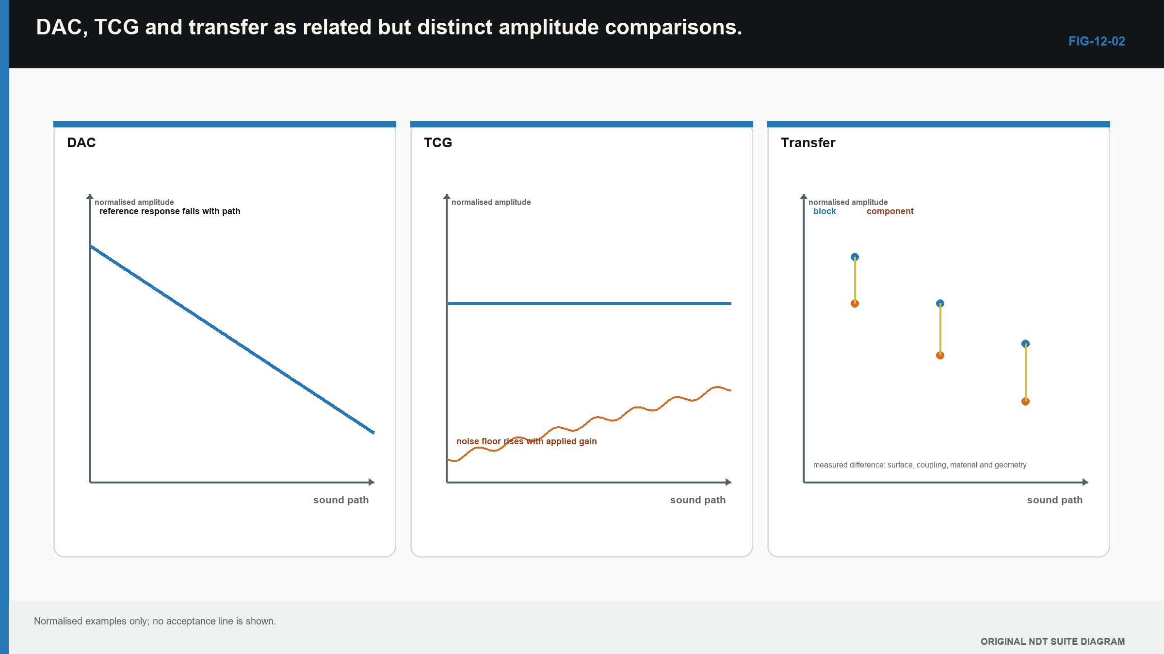
Notice that DAC changes the comparison line, TCG changes gain with time and transfer compares two physical paths.
| Worked example · Compare an indication with DAC WE-12-03 Given: At a 90 mm path, the DAC reference is 70% full-screen height. An unsaturated indication is 35% under the same processing. Find: The amplitude difference from DAC. Steps: Calculate the amplitude ratio and use 20 times the base-10 logarithm. difference = 20 log10(35/70) difference = 20 log10(0.5) = -6.02 dB Answer: The indication is about 6 dB below DAC at that path. What it means in practice: The result compares received amplitudes under the setup. It does not mean the reflector has half the diameter, area or length of the reference. Common mistake: Turning a 6 dB amplitude difference directly into a physical size difference. |
|---|
12.7 Scanning and evaluation sensitivity
Scanning sensitivity is selected to find relevant responses over the planned volume without unacceptable saturation or noise. Evaluation sensitivity is the controlled level used to compare and analyse an indication. They may differ.
Every gain change should remain traceable. If scanning uses extra gain, the record should show how the indication was returned to the comparison basis. A response clipped during scanning cannot be evaluated quantitatively from the clipped waveform.
Reserve gain describes available unsaturated amplification above a reference condition. There is no one useful reserve value for every instrument, path and target. The required margin follows expected signal range and technique purpose.
12.8 Transfer compares stated conditions
The reference block and component may differ in surface, curvature, attenuation and coupling. A transfer comparison estimates their response difference under controlled, comparable conditions.
| Worked example · Calculate a component-to-block transfer difference WE-12-02 Given: With the same probe, settings and comparable path, a reflector in the component simulation gives 38% screen height. The comparison block gives 60%. Find: Component response relative to block in decibels. Steps: Use an amplitude ratio. difference = 20 log10(38/60) difference = -3.97 dB Answer: The component response is about 4.0 dB lower under the compared conditions. What it means in practice: This supports a correction estimate for the stated path, surface and setup. It does not prove an intrinsic material attenuation value or justify the same correction everywhere. Common mistake: Adding 4 dB as unexplained extra scanning gain and applying it to every angle and depth. |
|---|
Several comparison positions can reveal whether one correction is reasonable. Values of -2, -3 and -4 dB suggest a different situation from -1, -3 and -10 dB. The wide value may indicate local coupling, roughness or material structure that a single average would hide.
12.9 Check stability before, during and after the work
A pre-check establishes the starting state. A post-check tests whether important properties remained within the permitted range. Extra checks may be needed after a knock, temperature change, probe replacement or other event likely to affect the system.
Check timing should follow the likely drift. A wearing hot wedge can change faster than a stable immersion arrangement. A continuous reference channel may show changes during an encoded scan, while pre/post checks only bound the interval.
The check should be sensitive to the property that matters because a stable reference peak does not prove stable index or angle. A correct distance point does not prove useful signal-to-noise, and one convenient saved screen should not be asked to certify the entire setup.
12.10 Respond to a failed final check
A failed check does not make every earlier observation imaginary. It also cannot be ignored. The response follows four practical steps:
- Identify which property changed: time, angle, index, amplitude, noise or another controlled value.
- Preserve the failed state and confirm the observation without casually resetting it.
- Determine the possible affected interval using earlier checks, retained references and scan evidence.
- Decide which data depend on the changed property and what must be repeated.
A constant time shift threatens location and thickness. An amplitude loss threatens threshold and amplitude comparison. An angle or index change threatens both coordinates and coverage. Increased noise can threaten detection while the main reference echo remains visible.
Formal calibration fitting and uncertainty analysis continue at Level 3. At Level 2, the essential skill is to separate the controls, recognise their visible failure and keep the result inside the evidence.
General UT principles do not supply one universal scan extent or acceptance rule for every product. Application documents provide those requirements. [R041] The practical calibration sequence in this chapter remains grounded in the cited international training foundation. [R001]
In plain words
- Time base, probe behaviour, reference amplitude and application performance are separate controls.
- Two distance points can separate a scale error from a constant offset.
- Actual probe index and angle matter more than the wedge label.
- DAC, TCG and DGS are controlled amplitude-comparison tools.
- A reference echo does not prove flaw type, flaw size or complete coverage.
- Transfer belongs to a stated comparison path and condition.
- A failed final check requires impact review tied to the property that changed.
Key terms
- Time-base calibration: checking displayed distance against known paths.
- Reference sensitivity: a controlled amplitude comparison.
- DAC: measured reference response versus distance at fixed gain.
- TCG: path-dependent gain used to flatten a reference family.
- DGS: model-based comparison with ideal reflectors.
- Transfer: a specific reference-to-component difference.
- Drift: change in system response during the inspection interval.
Key relationships
- d_display = a d_true + b separates scale and offset in a simple linear model.
- dB = 20 log10(A2/A1) compares two unsaturated amplitudes.
- A useful reference relationship includes target, path, probe, processing and surface conditions.
Common mix-ups
- One aligned echo is not a complete time-base calibration.
- Reference sensitivity is not application qualification.
- TCG does not reduce material noise; it raises late noise with the reference.
- Transfer correction is not arbitrary extra gain.
- A satisfactory amplitude check does not prove angle, index or data coverage.
Bridge to Chapter 13
Chapter 12 established where echoes appear and how amplitudes are compared. Chapter 13 uses those controlled values to plan real beam paths through a component. It turns weld drawings, probe positions and scan spacing into a visible coverage argument.
Sources and further study
- [R001]
- [R010]
- [R041]
Study and revision only. This is not an approved inspection procedure, acceptance criterion or qualification.