
CHAPTER 57 · FMC / TFM / PCI Level 3
Acoustic Models for Interfaces, Layers and Anisotropy
In this chapter · 26 sections
Why this matters
An image can be sharply focused and still put a reflector in the wrong place. This happens when the reconstruction predicts the wrong travel time. A wrong wedge angle, surface profile, layer thickness, wave speed or material direction can move the calculated response even when the instrument and stored samples are healthy.
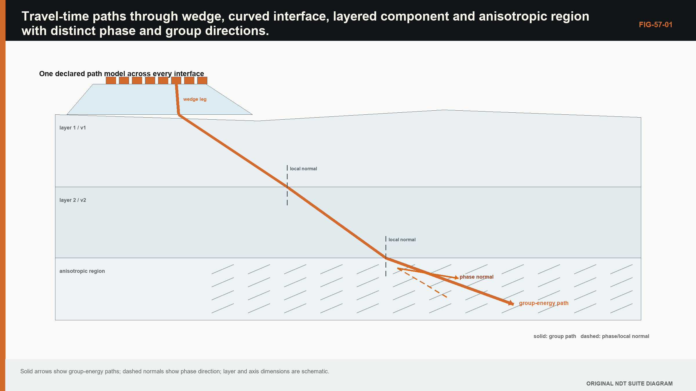
Begin with a simple error. A pulse crosses a wedge and then steel, but the reconstruction treats the whole path as steel. The predicted arrival is early, so the algorithm selects the wrong part of each A-scan and the reflector shifts or defocuses. A planar interface adds one crossing point. Several layers add several segments. Curvature changes the surface normal along the path. Anisotropy adds the further fact that energy direction and phase direction need not be the same.
What you already need
- Travel time equals the sum of time spent along each path segment.
- Refraction changes direction when wave speed changes across an interface.
- A TFM pixel depends on predicted transmit and receive travel times.
- Coordinates must identify the wedge, component and scan frames consistently.
What you will learn
You will build travel time from path segments; explain why an interface crossing may need to be solved rather than guessed; compare planar, layered, curved and anisotropic models; recognise localisation bias caused by a model error; and separate solver verification from validation against measured evidence.
Words you will meet
A path model describes the route and modes used to predict travel time. Root finding is a numerical search for the interface point that satisfies the path condition. Slowness is reciprocal wave speed and is useful when speed depends on direction. Group direction is the direction in which wave energy travels. Registration is the controlled relationship among coordinate frames.
The Level 3 step
At Level 2 a learner selects a declared path. At Level 3 the learner must decide whether that path model represents the actual wedge, interfaces and material well enough for the claimed location or size. The solver can be sophisticated, but its credibility still begins with visible position error on known reflectors and a clear record of the geometry and velocity used.
57.1 Travel time is a path-dependent model output
Every reconstructed pixel requires predicted transmit and receive travel times. In a homogeneous isotropic medium, straight-line distance divided by speed is sufficient. Interfaces, curvature, layers and anisotropy turn travel time into an optimisation or boundary-value problem. The solver must choose a mode sequence and a physically admissible path.
Fermat's principle states that the physical ray path is stationary in travel time with respect to small path variations. At a planar isotropic interface, this produces Snell's law. At curved or layered interfaces, one or more boundary points are unknown and solved by minimising or stationarising total time.
The path with minimum time is not always the only relevant arrival. Multiple stationary paths, mode conversions and reflections can exist. A solver that returns one number without path identity hides ambiguity. The reconstruction should retain mode and boundary sequence as part of the view definition.
57.2 Planar interfaces and root finding
For a two-medium path from source (x_s,z_s) to target (x_t,z_t) across a horizontal interface, let q be the lateral crossing coordinate. Total time is wedge distance to q divided by wedge speed plus component distance from q to target divided by component speed. The derivative with respect to q is zero at the stationary path.
| (57.1) Stationary two-medium travel time · EQ-57-01 Where: q = interface crossing coordinate; h_w = source height above interface; z_t = target depth below interface; c_w and c_m = represented mode speeds Model limits: planar interface, homogeneous isotropic media, one transmitted mode and a path confined to the declared plane |
|---|
Bisection is robust when a sign-changing derivative bracket is known. Newton methods are faster near the solution but can diverge or converge to the wrong stationary point. A production solver should define bracketing, tolerances and failure behaviour. Silently clipping an invalid path to an endpoint creates plausible but nonphysical travel times.
Independent checks include Snell-angle agreement, symmetry cases, normal incidence and comparison with a dense time scan. Units and coordinate signs should be tested explicitly.
57.3 Curved interfaces
A curved interface is parameterised by one or two surface coordinates. The solver finds a point whose path satisfies stationary time and geometric constraints. Surface normals vary, so local incidence and refraction change with position. Multiple solutions can appear for concave surfaces.
The surface representation matters. A nominal radius, measured profile, CAD mesh and local polynomial have different uncertainties. Interpolation of a coarse mesh can create normal discontinuities that translate into path jumps. Smoothing may improve numerical stability while removing real shape. The model choice should match the coordinate claim and be validated on known geometry.
Probe contact and stand-off add uncertainty. If the actual wedge position differs from registration, a mathematically exact curved path is still wrong. Surface finding and scanner metrology belong in the model input chain.
57.4 Multiple layers
For K isotropic layers, total time is the sum of leg lengths divided by mode speeds. Boundary crossing points are coupled because changing one alters adjacent legs. Snell's parameter is constant across planar parallel layers for a fixed mode sequence, providing an efficient solution.
Thin layers can also create interference and guided behaviour that geometric rays omit. A travel-time-only model may locate the first arrival while failing amplitude and phase. Whether that matters depends on reconstruction functional and layer thickness relative to wavelength.
Layer identity should be retained with travel time. A cladding-longitudinal to base-shear path is different from all-longitudinal. Software labels that abbreviate both to one view can cause interpretation errors.
57.5 Mode conversion and path families
At an elastic interface, incident energy can produce reflected and transmitted modes. A path model selects a sequence such as wedge longitudinal, component shear, backwall reflection and receive shear. Each leg has velocity and polarisation. Boundary coefficients influence amplitude, although many delay-only reconstructions ignore them.
Multi-mode TFM research uses direct, reflected and mode-converted paths to improve sensitivity to different target orientations. [R018] Multi-view analysis shows these paths also carry distinct artefacts and structural-noise behaviour. [R019] A broad view set can improve evidence only when each path is physically admissible and validated.
Path degeneracy occurs when different sequences have similar travel times in part of the ROI. Responses can map into plausible but wrong locations in multiple views. Geometry features are particularly prone to this. Cross-view convergence should include waveform and boundary behaviour, not coordinate coincidence alone.
57.6 Anisotropic slowness and group direction
In anisotropic elasticity, the Christoffel equation gives phase velocities and polarisations for a wave-normal direction. Slowness surfaces describe reciprocal phase velocity. Group velocity is normal to the slowness surface and gives energy direction. It can differ substantially from phase direction.
At an interface, tangential wavevector is conserved. The transmitted phase direction is selected from the slowness surface, then group velocity determines the ray path. Multiple quasi modes may satisfy the boundary condition. An isotropic Snell solver with an angle-dependent scalar speed can violate this relationship.
NASA analytical-ultrasonics work emphasises quasi modes and differences between group and phase direction in composites. [R006] Austenitic-weld evidence likewise shows direction and polarisation dependence. [R008] The material coordinate frame and elastic constants must be transformed consistently with the component geometry.
57.7 Registration among wedge, component and material frames
Three frames may be needed: array or wedge coordinates, component geometry and material orientation. In a weld, material axes can vary spatially. A rotation error changes anisotropic velocity even if component position is correct.
Registration data may come from CAD, scanner pose, surface measurements or a weld model. Each has uncertainty and version. A reconstruction recipe should identify the exact geometry and orientation field used. Editing a CAD mesh without changing a model identifier breaks provenance.
Known geometric reflectors can test combined registration and travel time. Agreement at one location may not validate varying curvature or material orientation. Multiple depths, positions and paths provide stronger evidence.
57.8 Model error and localisation bias
Travel-time error causes defocus and location bias. A common offset can shift all pixels; pair-dependent error reduces coherent sum. Velocity-scale error often produces depth-dependent bias. Wrong interface geometry produces position-dependent effects. Anisotropic direction error can create asymmetric blur.
Residual moveout is a useful diagnostic. At the image point selected as a target, extract contributing trace samples around predicted time. If peaks align systematically with element or offset, the model is incomplete. Adjusting parameters to flatten moveout is a form of model calibration and requires independent validation.
Uncertainty can be propagated by perturbing speeds, geometry and registration, then recomputing paths and images. The output may be a coordinate distribution, focus metric or detection statistic. Nonlinear solvers can jump between path branches, so distributions may be multimodal rather than Gaussian.
57.9 Solver verification and validation
Verification cases should have known answers: homogeneous distance, normal incidence, planar Snell refraction, symmetric layers and reversible paths. Mesh refinement or tolerance studies test numerical convergence. Reciprocity checks compare reversed endpoints under reciprocal assumptions.
Validation compares measured arrivals and images on representative materials and geometries. Travel-time agreement alone does not validate amplitude. A model intended only for delay reconstruction may not need perfect amplitude prediction, but target focus and artefacts should be examined.
The public scope of ISO FMC/TFM guidance recognises general use and related technologies while retaining application boundaries. [R047] A solver's inclusion in software does not establish its range. The validation record does.
| Worked example · Normal-incidence time through two layers WE-57-01 Known: A one-way normal path contains 10.0 mm of wedge at 2,730 m/s and 30.0 mm of component longitudinal path at 5,900 m/s. Find: One-way and pulse-echo travel times to a planar reflector at the end of the component leg. Method: Wedge time is 0.010/2,730 = 3.663 microseconds. Component time is 0.030/5,900 = 5.085 microseconds. One-way total is 8.748 microseconds; pulse-echo time is 17.496 microseconds. Result: Predicted one-way time is 8.75 microseconds and two-way time is 17.50 microseconds. Engineering meaning: This is a solver benchmark for normal incidence. Oblique paths require boundary-point solutions, and anisotropic paths require phase and group-direction treatment. |
|---|
Guided Level 3 case: a reflector that moves with the model
A known reflector is machined at a surveyed position below a curved component surface. A reconstruction using one nominal velocity places it 3.2 mm too deep and 1.5 mm to one side. Increasing gain sharpens the response but does not correct the coordinate. The fact that position changes when the model changes points toward travel-time or registration error rather than a simple sensitivity problem.
Begin with the least complex credible model. Confirm the probe and scan coordinates, the surface profile and the wedge reference. Reconstruct a nearby reference reflector using the same direct path. If both reflectors shift in a similar direction, a common coordinate or timing error is plausible. If the shift grows with depth or surface slope, the interface or velocity model becomes more likely.
Replace the single-medium assumption with a wedge-plus-component path through the measured surface. The solver searches for the interface crossing that makes the total path stationary for the declared modes. Its result must stay on the physical surface and inside the aperture. A converged numerical root outside the component is a mathematical result, not a valid acoustic path.
Now perturb the inputs one at a time. Change wedge delay within its measured uncertainty, change component velocity within the bounded material range and perturb the registered surface. Plot the reconstructed coordinate against each input. This identifies the variable that controls the observed bias and shows whether a single tuned value merely forces agreement at one reflector.
Validation uses more than the target that motivated the correction. Apply the model to reflectors at different depths, surface slopes and lateral positions. If one fitted velocity aligns the first reflector but misplaces the others, the model is absorbing geometry, anisotropy or registration error into an artificial property. A layered or directional material description may be required, or the technique boundary may need to exclude that region.
The release record contains the coordinate frames, interface data, mode sequence, velocity evidence, solver tolerance, invalid-path rules and residual position errors over the validation set. The conclusion is deliberately bounded: the revised model reduces localisation bias within the demonstrated region and conditions. It does not prove that every response in the component follows the same path family.
57.90 Technical extension: path-solver credibility in difficult media
57.90.1 Slowness-domain construction
For a fixed frequency, a slowness surface relates wave-normal direction to phase slowness. At an interface, the tangential component of slowness is conserved. Candidate transmitted modes are intersections of that tangential value with material slowness surfaces. Group velocity, normal to the surface, selects the direction carrying energy away from the interface.
This construction distinguishes a mathematically allowed phase solution from a physically incoming or outgoing energy branch. It also shows critical directions and cusps where small input changes produce large group-direction changes.
57.90.2 Elastic-constant uncertainty
An anisotropic solver may require density and a stiffness tensor. These quantities vary with material and orientation and can be difficult to measure locally. Symmetry reduces independent constants, but assuming the wrong symmetry creates model bias.
Perturb stiffness within evidence-based bounds and examine travel time, path and focus. The output sensitivity indicates which constants need better characterisation. Fitting many constants to limited travel times is underdetermined and should use physical constraints.
57.90.3 Spatially varying orientation
Weld models often define an orientation field from solidification assumptions. Rays then curve because local group direction changes. Numerical integration updates position and slowness through the field. Step size and interpolation of orientation affect accuracy.
The orientation field should be versioned and registered to actual weld geometry. A generic map centred on the nominal weld can be wrong after machining or repair. Macrographs or other material evidence can calibrate the field, with separate cases retained for validation.
57.90.4 Multiple stationary paths
Curved or layered components can admit several stationary paths between one element and pixel. A local Newton solver may return whichever branch is near its starting guess. Enumeration strategies use multiple seeds, continuation or global search, then remove duplicate solutions.
Each branch needs a physical validity and amplitude plausibility check. A later arrival may be relevant even when not minimum time. Reconstruction should identify branch and avoid switching silently across neighbouring pixels.
57.90.5 Boundary coefficients and polarisation
Delay-only imaging assumes all valid pairs contribute comparably after optional weights. In reality, transmission and reflection coefficients depend on incidence, mode and polarisation. Near critical conditions, amplitude can change sharply and phase can rotate.
Including coefficients can improve physical weighting but adds material inputs and convention. At minimum, paths with negligible expected transmission should not be counted as strong support. Coefficient models should be verified against limiting cases and validated experimentally.
57.90.6 Mesh and surface uncertainty
CAD meshes approximate surfaces with facets. Ray intersection and normals can jump at facet edges. Refinement should be guided by curvature and required timing accuracy, not a uniform triangle count. A smooth analytic surface provides a benchmark where available.
Measured surfaces include noise. Directly using every fluctuation can create nonphysical path jitter. Filtering needs a scale justified by surface metrology and wavelength. Retain both raw surface evidence and processed model.
57.90.7 Residual tomography
Travel-time residuals from known reflectors can be inverted for velocity or interface correction. This is a limited tomography problem. It can improve a model but may be non-unique: geometry and velocity changes can produce similar residuals.
Regularisation and prior bounds should be explicit. Corrected models are validated on hold-out paths. A residual fit that removes every error on calibration targets may overfit local noise.
57.90.8 Path uncertainty in interpretation
Where two path models remain plausible, reconstruct both and compare raw moveout, coordinate, morphology and independent features. Report conditional interpretations if neither is decisively supported. Choosing the sharper image alone favours the model that concentrates energy, including potentially wrong ones.
Path uncertainty can dominate coordinate precision. A cursor with 0.1 mm increments does not justify a 0.1 mm result when model alternatives differ by several millimetres.
57.90.9 Solver performance and caching
Complex path solving can dominate reconstruction. Precomputing travel times or using surrogate models improves speed. The cache key must include geometry, material, mode, element, grid and solver version. Interpolated surrogates need an error bound across path transitions.
Speed tests should include solver failures and branch handling. An implementation that silently falls back to a straight path can be fast and technically hazardous.
57.90.10 Validation matrix
Validation spans material directions, interface curvature, depths, paths and modes. Compare arrival time, energy direction, focal position and target response. No one target validates the whole solver.
The result should state where errors remain within the intended decision tolerance and where paths are excluded. [R004] [R006] [R008] [R018] [R019] [R047]
57.91 Travel-time residual acceptance
Define solver acceptance using observables rather than internal convergence alone. A root residual may be tiny while geometry inputs are wrong. Compare predicted and measured arrival times, interface points where observable, and focus across representative paths. Plot residual versus depth, angle and element offset to reveal structure.
When a correction model is fitted, report residual before and after, parameter covariance and hold-out performance. A smaller calibration residual is expected; the independent residual establishes useful improvement. [R004] [R006] [R008]
57.92 Path-model release controls
Release a path model with geometry and material hashes, coordinate conventions, mode sequence, solver tolerances, branch rules and validation range. Derived delay tables reference that identity. A change to any dependency invalidates cache reuse unless equivalence is demonstrated.
Runtime failures and excluded pixels should be counted and mapped. A smooth image created after silently replacing failed paths with zeros or straight-line times conceals lost support. [R006] [R008] [R047]
Chapter synthesis
Travel-time reconstruction is a path model. Interfaces and layers require stationary-time solutions; curvature makes surface representation part of the model. Mode-converted views need explicit leg and boundary sequences. Anisotropy requires slowness, polarisation and group-direction reasoning rather than a scalar velocity substitution. Wedge, component and material frames must be registered. Model errors appear as bias, residual moveout and loss of coherence. Solvers need analytical verification and application validation, with path identity and model version retained.
Key equations and relationships
| (57.2) Piecewise travel time · EQ-57-02 Where: T_P = travel time for declared path P; d_k = length of leg k; c_k = group or mode speed assigned to leg k Model limits: ray representation is adequate, each leg has a declared mode and material model, and boundary points satisfy the selected path physics |
|---|
In plain words
- The chapter's central control is path model, and its meaning must be stated before its mathematics or software implementation.
- A faster, sharper or cleaner result is not automatically a more reliable result.
- Every claimed improvement depends on a declared dataset, model, configuration and target population.
- Known reference cases and deliberately difficult cases reveal different weaknesses.
- Stored raw evidence, metadata and software identity make later review possible.
- The technical conclusion must remain inside the boundary demonstrated by the evidence.
Key terms in this chapter
The words introduced at the chapter opening are the minimum vocabulary for its Level 3 work. Use them consistently in the technique, validation record and report. Where a supplier uses a different label, record the supplier term without allowing it to replace the physical definition.
Common mix-ups
- Do not confuse a similar displayed image with equivalent retained information.
- Do not confuse software verification with physical validation of an inspection technique.
- Do not confuse an assumed model output with a directly observed quantity.
- Do not confuse a demonstrated result for one target population with universal capability.
Independent review checkpoint
Give a second competent reviewer the raw or reference data, the declared path model method, the controlled configuration and the expected comparison outputs. The reviewer should be able to reproduce the important result without using an undocumented display adjustment or private software setting. Record the version, input identity, contributor or channel mask, model inputs, numerical tolerances and any excluded cases. Also record one observation that would contradict the preferred explanation. Where the result supports a decision, the reviewer records the nearest failure boundary and one realistic change that would trigger revalidation. This checkpoint does not turn independent review into a ceremonial signature. It tests whether the evidence chain is understandable, repeatable and honest about its limits.
Bridge forward
Chapter 58 follows the predicted time into the sampled waveform and examines the numerical choices used to reconstruct an image.
Sources and further study
- [R004]
- [R006]
- [R008]
- [R018]
- [R019]
- [R047]
Study and revision only. This is not an approved inspection procedure, acceptance criterion or qualification.