
CHAPTER 16 · Ultrasonics Level 2
A Practical Interpretation Method
In this chapter · 20 sections
Why this matters
Interpretation goes wrong when the first plausible story becomes a fact. A repeatable echo may be a discontinuity, known geometry, a previous-pulse echo, a wedge response or a real reflector plotted using the wrong path. The safest answer comes from a sequence that starts with valid data and asks competing explanations to predict what will happen next. This chapter turns that reasoning into a practical Level 2 method. It does not require formal probability. It requires controlled observations, an honest record and a willingness to let a favourite explanation fail.
What you already need
- How to confirm calibration, coupling and unsaturated response.
- Basic reflector plotting and weld geometry.
- How translation, skew and a second angle change the sound path.
- The weld-response mechanisms from Chapter 15.
What you will learn
- How to separate false, non-relevant and relevant responses.
- How to use a repeatable interpretation funnel.
- How to test one physical cause at a time.
- How to weigh supporting, negative and duplicated evidence.
- How to record observation, interpretation and evaluation separately.
Words you will meet
- False response: a signal caused by equipment, processing or a wrongly assumed path rather than the plotted component location.
- Non-relevant response: a real component response outside the condition sought by the examination.
- Relevant response: a response plausibly connected to the condition the examination covers.
- Hypothesis: a physical explanation that can be tested.
- Corroboration: additional evidence that supports an explanation.
- Contradiction: evidence that does not behave as the explanation predicts.
- Data lineage: the link between a displayed view and the acquisition that produced it.
16.1 Start by proving the data are usable
Interpretation cannot repair invalid acquisition. Confirm the file or scan identity, setup, calibration state and probe position. Check coupling, range, gate placement and any encoder. Make sure the signal is not clipped by receiver or display saturation. Review reference and back-wall behaviour where those checks apply.
If a check fails, preserve the data but reduce the weight given to it. Do not silently correct an echo until it reaches the expected position. Record what failed, repeat under a valid state if possible and keep the two acquisitions distinct.
The working order is important: validity, detection, location, characterisation, sizing, then evaluation. Acceptance criteria should not decide whether the signal exists or what caused it. A rejectable-looking response can create pressure to overcall; a production-friendly response can create pressure to dismiss. The data should survive either pressure.
16.2 Use three response classes carefully
A false response comes from the system, processing or an unintended path. Examples include electrical noise, cross-talk, previous-pulse wrap-around, wedge reverberation and an echo plotted as all-shear when its path changed mode.
A non-relevant response is real sound from the component but is not caused by the condition being sought. A confirmed counterbore or a plate edge may be non-relevant for one examination. Relevance depends on the task: a root response may be relevant when root condition is part of the examination.
A relevant response plausibly comes from the population covered by the examination. Relevant does not mean rejectable, and it does not by itself identify a crack. Classification should follow evidence, not screen appearance. Known geometry can also coexist with a discontinuity, so explaining one part of a response does not automatically explain every nearby signal.
16.3 Work through the interpretation funnel
Use the same sequence for each response:
- Confirm data identity, calibration, coupling and unsaturated display.
- Check whether time and position fit the selected mode, leg and surface.
- Compare the result with as-built geometry and material history.
- Observe controlled translation, orbital movement and skew.
- Add a useful second angle, side, surface, mode or method where justified.
- Record evidence that supports and contradicts each live explanation.
- State the conclusion at the strength the evidence permits.
Each stage should remove explanations only when they fail a real prediction. The funnel narrows possibilities; it does not turn uncertainty into certainty by diagram.
The following figure shows the order in which the interpretation funnel narrows those explanations.
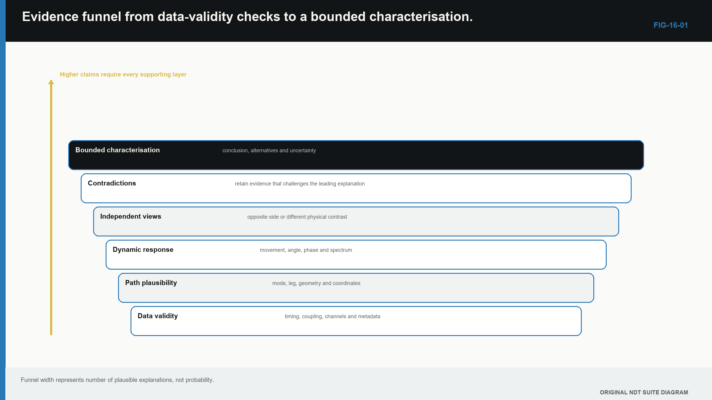
Notice that data validity and path plausibility are tested before characterisation language becomes specific.
16.4 Test path and geometry first
Plot the response in a declared component coordinate system. Write down the assumed wave mode and leg. Compare it with measured thickness, root, cap, backing, counterbore, plate edge and attachments. If the location depends on an assumed drawing dimension, keep that dependency visible.
Common traps make predictable changes. An edge echo should change as the probe moves relative to the edge. A fixed wedge echo stays at a probe-related time even when the proposed component path changes. A mode-converted path should fit the sum of its segment times. A previous-pulse echo should respond to pulse repetition frequency.
Change one causal variable at a time and predict the result before making the change. Randomly adjusting several controls until an echo disappears only creates a new setup. It does not explain the old response.
| Worked example · Identify a previous-pulse response WE-16-01 Given: A late echo remains at the same screen position while the probe moves over uniform plate. It disappears when pulse repetition frequency is reduced from 2,000 Hz to 500 Hz. The reference and back-wall echoes remain stable. Find: The leading response class. Steps: A local reflector should change with probe position. The late response does not. Its controlled dependence on pulse repetition frequency is expected when energy from an earlier pulse enters the current display window. Answer: Previous-pulse wrap-around is the leading false-response explanation. What it means in practice: The echo should not be plotted as a component indication. The conclusion is supported by one controlled change while genuine echoes remained stable. Common mistake: Removing the response by changing range and never determining why it appeared. |
|---|
16.5 Choose a check that separates explanations
A useful check makes the competing explanations behave differently. Suppose an echo could come from the wedge or from a reflector in the plate. Move to a place where the component path would change while holding the instrument settings and probe assembly constant. The wedge explanation predicts fixed probe-related time. The component explanation predicts a geometry-related movement or loss when the beam no longer meets it.
| Worked example · Choose a discriminating observation WE-16-04 Given: A response could be a fixed wedge echo or a component reflector. At two initial component positions it appears at the same screen time. Find: A check that makes the explanations predict different outcomes. Steps: Keep the setup fixed and move the probe to a region where the path to the proposed component reflector must change. Track echo time and the plotted component coordinate. Answer: Time fixed to the probe supports the wedge explanation. Movement consistent with component geometry supports the component-reflector explanation. What it means in practice: The check is valuable because it separates causes, not simply because more data were collected. Common mistake: Changing gain, range, probe and position together, leaving no single cause to interpret. |
|---|
Use the same approach for a weld-root versus fusion-face explanation. Choose an angle or surface for which their predicted positions or directional strengths differ. Before relying on a quiet second view, prove that the view had enough sensitivity and suitable orientation for the target.
16.6 Record observation before inference
Separate three layers in the notes.
Observation states what was measured: screen time, corrected coordinate, amplitude behaviour, response extent, probe movement, angle, side and data quality. Interpretation states which reflector or path models those observations support and which alternatives remain. Evaluation applies the governing acceptance basis after the interpretation is complete.
This separation makes review possible. Another analyst can disagree with the physical model without losing the original observations. It also prevents an acceptance threshold from being mistaken for a detection threshold.
Useful language has different strength. “Observed” belongs to the data. “Consistent with” means an explanation fits but is not unique. “Supports” means distinct evidence favours it. “Demonstrates” should be reserved for a relationship actually established within stated bounds.
| Worked example · Characterise a response without overclaiming WE-16-02 Given: An indication is repeatable on a modelled fusion face, strongly directional, visible from both sides with different amplitudes and accompanied by two weak extremity-like responses separated by 4.5 mm. Data are unsaturated and position checks are valid. Find: A defensible characterisation statement. Steps: State the observations, the favoured physical model and the unresolved limits. Do not convert an acoustic pattern into a proven metallurgical type. Answer: “A repeatable directional response is located on the modelled fusion face. Opposite-side response and two separated extremity signals support a planar-reflector hypothesis with an indicated extremity separation of about 4.5 mm. Reflector type and true height remain subject to the stated path and tip-identification limits.” What it means in practice: The statement gives engineering-useful evidence without claiming more than the data support. Common mistake: Reporting “4.5 mm lack of fusion” as though location, type and true size had all been proved by one display. |
|---|
16.7 Weigh corroboration, duplication and absence
Evidence becomes stronger when another observation has different failure modes. Opposite-side scanning changes coupling and path, although it may share the same geometry model. A different angle changes target incidence but may share surface and calibration. A complementary method can use another physical contrast while still relying on common coordinate truth.
Three views drawn from one acquisition are useful views, not three independent detections. In common encoded data, the A-scan is the waveform, the B-scan is a side view and the C-scan is a plan view. They can share probe, coupling, timing and raw waveform, so counting them separately inflates confidence. Track data lineage so every displayed image can be traced to its physical acquisition.
The following dependency figure makes those shared and separate failure causes visible.
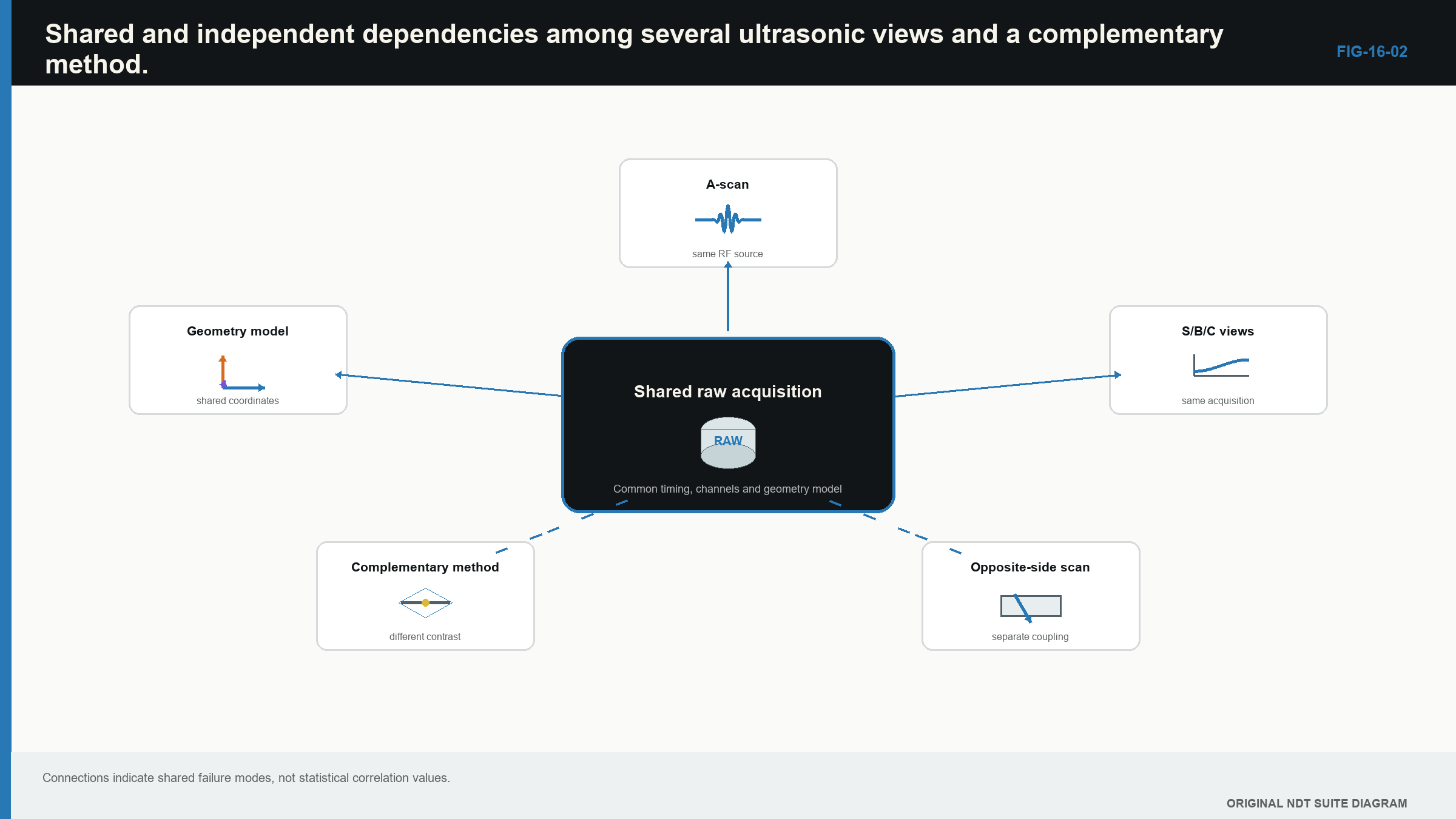
Notice that three displays can remain one physical acquisition, while a separately acquired path adds different evidence.
| Worked example · Do not count three displays as three detections WE-16-03 Given: A response appears on A-, B- and C-scan views from one encoded acquisition. A separate opposite-side scan does not show it, but that scan demonstrates only 1 dB signal-to-noise ratio for the relevant target orientation. Find: Whether the evidence is three positive results against one negative result. Steps: The three displays share one raw acquisition. They provide one positive physical observation viewed three ways. The opposite-side absence comes from a path with weak demonstrated sensitivity, so it is inconclusive rather than strong negative evidence. Answer: The evidence is one positive acquisition plus one inconclusive second acquisition. What it means in practice: Acquisition lineage and capability control evidential weight, not the number of images in the report. Common mistake: Treating every reconstructed view as an independent confirmation. |
|---|
Absence matters only when the path could have found the proposed target. If a suitable representative target is clearly detected at that location and orientation, a missing indication can weaken the hypothesis. If coverage or signal-to-noise ratio is unknown, “not seen” means little.
16.8 Control human bias
Expectation affects what people notice. A seeded-flaw location can make noise look meaningful. A previous report can anchor position and size. Schedule pressure may favour geometry; fear of missing a crack may favour overcalling. These influences are part of the measurement system even when the analyst is experienced.
Practical controls include recording the initial observation before reading prior conclusions, requiring at least one alternative explanation and using an independent review for significant calls. A reviewer needs underlying data, setup identity and coordinate model. Reviewing only an annotated screenshot inherits the first analyst’s selection.
Automation does not remove bias. A detector can make analysts trust highlighted regions and neglect others. Its missed and false-call patterns must be evaluated as part of the combined human and system process.
16.9 Investigate a suspected false call without erasing it
Preserve the original configuration and response. Establish its screen time and component coordinates, inspect the least-processed available data and check reference channels. Then vary one diagnostic control with a predicted outcome.
If reducing pulse repetition frequency removes a late echo, record both repetition rates and the timing relationship. If replacing a cable removes an electrical spike, the evidence supports a system-origin explanation. It does not prove which connector failed unless that cause is separately inspected or measured.
Contradiction is useful. If a proposed root echo does not follow measured root geometry, the root model weakens. If a planar face should respond strongly from a proven second view and does not, that model weakens. Do not hide the contradiction; explain what it changes.
16.10 State the conclusion and its limit
A useful result includes response class, corrected position, observed behaviour, favoured physical explanation, evidence used and material limitations. Limits may include inaccessible coverage, poor structural signal-to-noise ratio, unresolved extremities, uncertain geometry, anisotropic location error or one invalid acquisition.
A limitation does not make the examination useless. It marks where the conclusion ends. If two explanations remain plausible, reporting the unresolved alternatives may be the technically strongest result.
Formal updating of prior likelihoods and evidence belongs to Level 3 and Part VIII. The original Bayesian relationship is preserved for that treatment as EQ-16-01. At Level 2, the sound habit is simpler: ask what each explanation predicts, seek an observation that separates them and reduce confidence when the prediction fails.
The interpretation foundation in this chapter remains consistent with the international UT training reference. [R001]
In plain words
- Valid data come before interpretation.
- False, non-relevant and relevant describe supported response classes, not screen shapes.
- Plot the path and compare actual geometry before naming the cause.
- Change one variable and predict what each explanation should do.
- Record observations separately from interpretation and acceptance evaluation.
- Several displays from one acquisition are not several independent detections.
- A quiet view is useful negative evidence only when its capability was demonstrated.
- State unresolved alternatives and limits instead of forcing certainty.
Key terms
- Interpretation funnel: an ordered way to narrow competing physical explanations.
- Independent evidence: evidence whose important failure causes are not all shared with the first observation.
- Negative evidence: a missing response from a path proven capable of showing the proposed target.
- Disconfirming check: a test selected because a proposed explanation predicts a particular outcome.
- Bounded conclusion: a conclusion that states where its evidence and model stop being reliable.
Key relationships
- Validity precedes detection, location, characterisation, sizing and evaluation.
- Evidence weight depends on physical independence and demonstrated capability, not display count.
- A useful diagnostic change is one for which competing causes predict different outcomes.
- Formal probabilistic hypothesis updating is relocated as EQ-16-01; routine Level 2 work uses the same discipline without unsupported numbers.
Common mix-ups
- Repeatable does not automatically mean relevant; component geometry is repeatable too.
- Relevant does not automatically mean rejectable.
- A response below threshold is not proof that a target is absent.
- Reprocessing one waveform does not create new physical evidence.
- Confidence in a statement is not evidence for the statement.
Bridge to Chapter 17
Once a response is valid, located and characterised as far as the evidence permits, the next task may be sizing. Chapter 17 explains what common sizing methods actually measure, how to match a method to the signal and how to report uncertainty without burying the practitioner under advanced mathematics.
Sources and further study
- [R001]
Study and revision only. This is not an approved inspection procedure, acceptance criterion or qualification.