
CHAPTER 58 · FMC / TFM / PCI Level 3
Reconstruction Algorithms, Interpolation and Computation
In this chapter · 27 sections
Why this matters
The travel-time model rarely lands exactly on a stored sample. If a trace is sampled every 10 nanoseconds and the predicted arrival is 104 nanoseconds, the required value lies at sample index 10.4. The reconstruction must estimate the waveform between samples. That estimate is called interpolation, and it can change phase, amplitude, location and coherence.
This small example is the entrance to reconstruction computation. The same result can also change through pixel spacing, analytic-signal order, numerical precision, summation order, lookup-table rounding or parallel hardware. Faster code is valuable only when the numerical behaviour is understood and the important output remains within a demonstrated tolerance.
What you already need
- A digitiser stores waveform values at regular time intervals.
- A travel-time model predicts a time for each trace and trial pixel.
- TFM combines many selected values, so small errors may accumulate.
- A reconstruction setup includes an ROI, grid, aperture and path model.
What you will learn
You will calculate a fractional sample index; apply and limit linear interpolation; explain why processing order matters; estimate how grid points and trace count change computational work; distinguish speed from numerical equivalence; and define regression tests for a controlled implementation.
Words you will meet
Fractional delay means that the required waveform time lies between stored samples. Interpolation estimates a value between samples. An analytic signal combines the waveform with a quadrature component so envelope and phase can be calculated. Determinism means the same controlled input produces the same output within a declared numerical rule. A regression test checks that a software change has not altered an established result unexpectedly.
The Level 3 step
At Level 2 the learner sees that grid spacing and sample rate affect an image. At Level 3 those effects become part of a numerical error budget. CPU and GPU detail is included only after the learner can explain the fractional-sample problem, because hardware vocabulary is not a substitute for understanding the calculation.
58.1 Reconstruction is a numerical experiment
An imaging equation becomes an algorithm through sampling, interpolation, filtering, data layout, arithmetic and parallel execution. These choices can change amplitude, phase, localisation and runtime. They are not merely software details when the image supports a technical decision.
A reproducible reconstruction identifies input bytes, metadata, preprocessing order, travel-time solver, grid, functional, weights, normalisation, arithmetic precision, software version and hardware-sensitive options. Repeating the same acronym on the same computer is not enough if hidden defaults can change.
Frequency-domain imaging can provide major speed benefits for regular geometries, while time-domain approaches are flexible. Comparative research shows that algorithm performance and artefacts depend on sampling and interpolation parameters as well as material noise. [R020] [R021] A benchmark must therefore compare technical outputs and computational conditions, not only elapsed time.
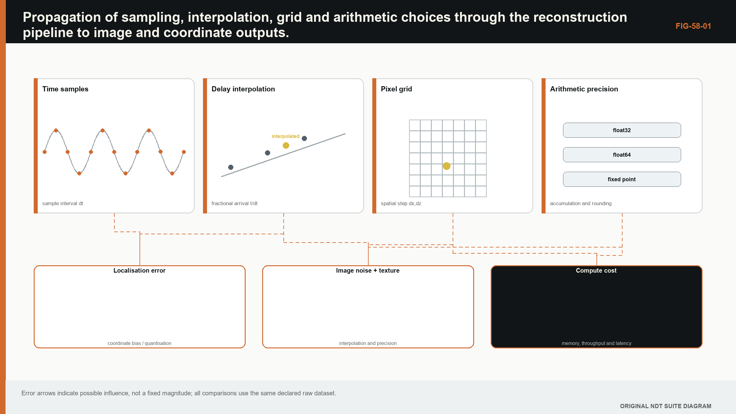
58.2 Time sampling and fractional delays
At sampling rate f_s, stored samples are separated by Delta_t = 1/f_s. Predicted travel times generally fall between samples. Nearest-neighbour selection is fast but creates timing quantisation up to half a sample. Linear interpolation reduces discontinuity but attenuates high-frequency content relative to an ideal bandlimited interpolator. Higher-order polynomial or sinc interpolation can improve accuracy while increasing computation and edge sensitivity.
Sampling theory states that a bandlimited signal can be reconstructed when sampling exceeds twice its highest frequency and the anti-alias condition is met. [R005] Real ultrasonic pulses are not perfectly bandlimited, and analogue filtering determines what reaches the digitiser. Oversampling provides interpolation margin but does not restore frequencies removed or aliased before storage.
| (58.1) Linear interpolation at a fractional sample · EQ-58-01 Where: n = floor(t/Delta_t); a = t/Delta_t - n; Delta_t = sample interval; x[n] and x[n+1] = neighbouring stored samples Model limits: local signal is adequately represented by a straight segment and both neighbouring samples are valid |
|---|
Interpolation should be verified with known waveforms over fractional delays. Peak error, phase error and group delay across the relevant band are more informative than one time-domain trace. Near the start or end of a record, the interpolation kernel may extend beyond available samples; the algorithm needs a declared boundary rule.
58.3 Analytic signals and processing order
The analytic signal is commonly obtained by a discrete Hilbert transform or frequency-domain one-sided spectrum. Its magnitude gives an envelope and its angle gives instantaneous phase where amplitude is sufficient. Finite records, padding and filter design create edge effects.
Order matters. Filtering each trace before delay-and-sum is not always equivalent to filtering the image after summation, especially with nonlinear envelope or coherence operations. Rectifying before summation removes sign and changes interference. Normalising traces individually changes aperture weighting.
The processing graph should therefore be explicit. If raw RF is filtered, record filter type, coefficients, passband, phase response and padding. If an analytic signal is stored rather than computed, record implementation and relationship to raw samples.
58.4 Grid design
The ROI defines where the model is evaluated. Pixel spacing should sample the expected point-spread response and geometry adequately. A coarse grid can miss peaks or quantise boundaries. A very fine grid increases computation and creates visually smooth interpolation without improving physical resolution.
Adaptive grids can refine near features while remaining coarse elsewhere. Their output requires coordinate-aware storage and display; assuming a regular pixel size can distort measurements. Curvilinear grids may follow a component boundary and improve sampling efficiency, but distances in index space are not physical distances.
Grid origin is as important as spacing. Shifting a coarse grid by half a pixel can change a reported maximum. Grid-convergence studies reconstruct with successively finer or shifted grids and compare coordinates, amplitude and morphology. Convergence to a stable image does not prove the acoustic model, but it controls numerical discretisation.
58.5 Computational scale
Direct TFM work scales approximately with number of pixels times number of contributing pairs, plus interpolation and weighting. For a 100,000-pixel ROI and 4,096 pairs, one position requires about 410 million pair-pixel evaluations. Multiple paths, positions or parameter sweeps multiply the burden.
| (58.2) Direct delay-and-sum operation scale · EQ-58-02 Where: W = computational work proxy; N_pixel = reconstruction points; N_pair = contributing transmit-receive pairs; N_view = separately reconstructed path views Model limits: direct evaluation with similar cost per pair-pixel-view and no algorithmic reuse |
|---|
Operation count alone does not predict runtime. Memory movement, cache, interpolation access pattern and output writes can dominate. A GPU may execute arithmetic quickly but wait on irregular global-memory reads. Data layout that stores time contiguously per trace supports one access pattern; transposed layouts support another.
58.6 CPU, GPU and heterogeneous execution
CPUs offer flexible control, large caches and mature double-precision behaviour. GPUs offer massive parallelism when many pixels and pairs can be evaluated independently. Heterogeneous systems may compute travel times on CPU, reconstruct on GPU and post-process elsewhere.
Transfer between host and accelerator consumes time and can duplicate memory. For small images, transfer overhead can exceed compute savings. For large datasets, limited device memory may require tiling by pixels, pairs or positions. Tile boundaries should not change normalisation or filtering.
Hardware implementations can differ in floating-point contraction, transcendental functions and reduction order. These differences are often small but should be measured against technical tolerances. A bitwise-identical requirement may be unnecessary; an output-equivalence criterion with reference data may be appropriate.
58.7 Precomputed delays and lookup tables
Travel times can be precomputed for a fixed geometry and grid. This exchanges arithmetic for memory. A delay table also freezes the path model and should carry its own identity, units, element map and geometry version.
Quantised delay indices are smaller than floating-point times but may discard sub-sample information. Storing base index plus fractional weight supports linear interpolation. Higher-order kernels need more coefficients or on-the-fly calculation.
Reusing a delay table after changing velocity, wedge, probe position or grid is invalid even if dimensions match. Hashes and explicit dependency manifests can prevent accidental reuse. A cache key should include every input that changes travel time.
58.8 Numerical precision and summation
Single-precision arithmetic is often sufficient for sample values and many travel-time calculations, but path length, large coordinate origins or long sums can expose precision loss. Subtracting nearly equal large numbers to obtain a small offset is particularly sensitive.
Summation order changes floating-point rounding. Parallel reductions combine partial sums in an order that may vary. Kahan or pairwise summation can reduce error at additional cost. The significance grows when large positive and negative contributions nearly cancel, as in coherence-sensitive or sidelobe regions.
Precision should be tested with representative worst cases: long paths, fine grids, many channels, low residuals and large coordinate offsets. Reporting that a GPU uses 32-bit values is not an error analysis.
58.9 Parallelisation and determinism
Pixels are naturally parallel for a fixed view and position. Pairs can also be parallel but require reduction. Positions and views add higher-level parallelism. The design should avoid race conditions in shared outputs and keep pair validity consistent.
Deterministic execution returns the same result within a declared tolerance for identical inputs. Non-determinism can arise from reduction order, asynchronous streams, uninitialised memory or adaptive algorithms. A release build should distinguish harmless floating variation from unstable logic.
Thread count and GPU model can be recorded where they affect output. Performance benchmarks should include warm-up, transfer and I/O definitions. Selecting only the fastest run is not a reproducible benchmark.
58.10 Versioning and algorithm verification
Regression tests span levels. Unit tests verify interpolation, coordinate transforms and weights. Analytical tests verify homogeneous travel times and symmetry. Synthetic datasets test known point targets and noise. Golden datasets compare complete images and derived measurements.
Tolerance selection should reflect numerical expectations and technical consequence. Exact hash comparison is suitable for deterministic byte outputs. Numeric arrays may use absolute, relative or image-feature tolerances. A broad image-correlation score can hide a local coordinate shift, so key metrics should be explicit.
Open computational frameworks can support reproducibility, but software availability does not establish industrial validation. NASA's PanNDE record emphasises plugin architecture, metadata and V&V concepts. [R039] k-Wave provides well-known wave simulation capabilities under its own scope, not an automatic validated solid-UT reconstruction. [R040]
| Worked example · Fractional-sample interpolation and timing scale WE-58-01 Known: Sampling rate is 40 MHz, so samples are 25 ns apart. A predicted delay is 7.5375 microseconds, corresponding to index 301.5. Neighbouring RF samples are 0.40 and 0.70 in linear units. Find: Linear-interpolated value and direct longitudinal pulse-echo distance represented by half a sample at 5,900 m/s. Method: Interpolated value is 0.5(0.40) + 0.5(0.70) = 0.55. Half-sample distance scale is 5,900(12.5e-9)/2 = 0.0369 mm. Result: Linear interpolation gives 0.55; half a sample represents about 0.037 mm in the simplified direct pulse-echo distance model. Engineering meaning: Timing quantisation can be small in distance yet significant in phase. Interpolation error, path geometry and model bias can exceed the half-sample scale. |
|---|
Guided Level 3 case: a faster reconstruction changes the result
A GPU implementation reduces reconstruction time from forty seconds to three seconds. Most pixels agree with the CPU reference, but a small indication moves by 0.3 mm and its peak changes by 1.1 dB. The difference is small on the full image and large enough to matter near a measurement or reporting boundary. Performance alone cannot decide whether the change is acceptable.
Freeze one input dataset, travel-time table, ROI, contributor mask and display rule. Export numerical pixel arrays rather than comparing screenshots. Begin with a few selected pixels for which the contributing trace times and samples can be inspected manually. A predicted time of 10.4 samples should use the same interpolation convention in both implementations. One system may round to sample 10 while another linearly combines samples 10 and 11. That difference can alter phase before many contributions are summed.
Next isolate processing order. Confirm whether analytic signals are formed before interpolation, after interpolation or after summation. Confirm whether weights are applied to complex samples, RF samples, envelopes or energy. These operations do not generally commute. A method description that lists all operations but omits their order is incomplete.
Then test numerical precision and summation order. Parallel reduction can add thousands of floating-point values in a different sequence from a serial calculation. Use high-dynamic-range synthetic traces and cases with near cancellation, because easy coherent sums can hide the effect. Repeat the GPU calculation to establish whether it is deterministic under the declared hardware and library configuration.
Compare outputs at several layers. Record maximum and percentile pixel differences, target coordinate, peak response, point-spread width and any derived decision. Examine blank, single-target, multiple-target and artefact cases. A global mean error can be tiny while one critical region exceeds tolerance.
The final tolerance comes from measurement consequence, not coding convenience. If the 0.3 mm shift is below the demonstrated coordinate uncertainty and cannot change the stated decision, the implementations may be equivalent for that use. If it changes a threshold result or coherence feature, the new version needs correction or a separately validated definition. The release package stores reference inputs, expected numerical outputs, tolerances, software identity and the reason each difference is acceptable.
58.90 Technical extension: numerical error budgets and reproducible performance
58.90.1 Interpolation transfer functions
An interpolation kernel has a frequency response. Linear interpolation attenuates content near Nyquist and creates phase behaviour dependent on fractional delay. Sinc-like kernels approximate bandlimited delay but require finite windows. Plot amplitude and phase error across frequency and fractional offset to select a method for the actual bandwidth.
Testing only integer-sample delays misses the problem completely. A verification sweep should cover fractions from zero to nearly one sample and signals at several frequencies and phases.
58.90.2 Filter commutation
Linear time-invariant filtering commutes with summation under ideal complete records, but finite windows, channel-specific filters and delay interpolation can break equivalence. Envelope, clipping and coherence are nonlinear and do not commute.
Document order with a processing graph and test alternative orders on reference data. If outputs differ materially, order is an essential parameter rather than an implementation detail.
58.90.3 Time-origin precision
Large absolute timestamps represented in floating point can lose precision when a small delay is added. Store travel times relative to a local origin or use integer sample indices plus fractional parts. Coordinate origins likewise should be near the component region when possible.
Conversion among seconds, microseconds, millimetres and metres is a common defect source. Unit-aware tests and metadata reduce risk. A result can be numerically stable and wrong by a factor of one thousand.
58.90.4 Memory-layout verification
FMC arrays can be ordered as transmit-receive-time, position-transmit-receive-time or another layout. A transposition error may still produce a plausible image for symmetric targets. Use asymmetric pair impulses and element maps to verify axes.
Endianness and signedness should be tested with known byte patterns. Zero-copy or GPU transfers need explicit stride checks. A shape alone does not guarantee contiguous or correctly ordered data.
58.90.5 Mixed precision
Mixed-precision pipelines may store samples in integers, convert to 16- or 32-bit floats, compute delays in 32 or 64 bit and accumulate in another type. Each transition can saturate, round or lose dynamic range.
Compare worst-case outputs with a higher-precision reference. Focus on cancellation regions, long sums and small coordinate differences. A global image correlation can hide a local amplitude or position error.
58.90.6 Deterministic reductions
Parallel summation order varies when work scheduling changes. Pairwise tree reductions are more stable than arbitrary atomic additions. Deterministic kernels can aid regression at some performance cost.
Where bitwise determinism is not required, define numeric tolerances tied to technical outputs. Repeat runs across thread counts and hardware to establish variation. Intermittent large differences indicate a race or uninitialised data, not harmless rounding.
58.90.7 Performance models
Use roofline or arithmetic-intensity reasoning to determine whether a kernel is compute or memory bound. If each sample is read once for few operations, memory bandwidth dominates. Caching delay indices or reorganising pairs can help more than increasing arithmetic units.
Report end-to-end latency including input, transfers, reconstruction and output. Throughput in pixels per second without pair count and interpolation is not comparable across methods.
58.90.8 Scalability and tiling
Tiling over pixels preserves independent sums but can duplicate delay data. Tiling over pairs requires partial-image accumulation and consistent normalisation. Tiling over time may fail when interpolation kernels cross boundaries.
Tests should compare tiled and untiled reference outputs, including ROI edges and partial support. Memory-pressure fallbacks must not change algorithm silently.
58.90.9 Provenance of computational environments
Record source revision, build options, compiler, critical libraries, hardware and configuration. Containers can capture dependencies but not every driver or device behaviour. A reproducible recipe includes input hashes and expected metrics.
Long-term release should retain a simple reference implementation where possible. An optimised GPU kernel can be checked against a slower transparent calculation on small cases.
58.90.10 Release tests
A release suite includes unit, analytical, synthetic, golden-image, performance and fault tests. Fault tests provide missing metadata, invalid paths, NaNs, clipped data and out-of-range indices. The expected behaviour is explicit failure or flagged output, not a plausible default.
Test reports should be immutable release artefacts linked to software and datasets.
58.91 Computational release envelope
A reconstruction release should state supported data dimensions, paths, grid size, precision and hardware, plus failure behaviour outside that envelope. Stress tests at maximum dimensions should verify no integer overflow, index truncation or memory fallback changes the algorithm.
Performance claims should use sustained end-to-end datasets and report median and tail latency. A fast average with occasional multi-second stalls may violate an automated workflow. Output-equivalence tests across supported hardware protect technical results while allowing reasonable floating variation. [R020] [R021]
58.95 Engineering check: test interpolation away from convenient sample positions
Interpolation should be assessed with fractional delays distributed across the complete sample interval, not only with arrivals that happen to land close to stored samples. Synthetic band-limited pulses can expose amplitude, time and phase bias for each fractional position. The test is then repeated near trace boundaries and with the filters, decimation and analytic-signal processing used in production.
These results establish an implementation error scale that is separate from physical model error. If changing interpolation order moves an image peak materially, the reconstruction is not numerically converged for that task. The chosen method should be justified by the demonstrated error, computational cost and required output, rather than by a default library setting. [R016] [R023] [R024]
Chapter synthesis
Reconstruction output depends on sample interpolation, processing order, grid, data layout, arithmetic and execution. Sampling theory bounds recoverable time information, while fractional-delay interpolation affects phase and amplitude. Grid refinement controls numerical discretisation, not acoustic resolution. Direct TFM can be memory bound despite high arithmetic parallelism. Precomputed delays require dependency control. Floating precision, reduction order and determinism need measured tolerances. Layered verification and versioned regression datasets turn an algorithm into a reproducible measurement component.
Key equations and relationships
| (58.3) Sample-time index · EQ-58-03 Where: q = fractional sample index; T = predicted travel time (s); f_s = sampling rate (Hz); n = integer base index; a = fractional part in [0,1) Model limits: uniform sampling and a time origin consistent with the travel-time model |
|---|
In plain words
- The chapter's central control is fractional delay, and its meaning must be stated before its mathematics or software implementation.
- A faster, sharper or cleaner result is not automatically a more reliable result.
- Every claimed improvement depends on a declared dataset, model, configuration and target population.
- Known reference cases and deliberately difficult cases reveal different weaknesses.
- Stored raw evidence, metadata and software identity make later review possible.
- The technical conclusion must remain inside the boundary demonstrated by the evidence.
Key terms in this chapter
The words introduced at the chapter opening are the minimum vocabulary for its Level 3 work. Use them consistently in the technique, validation record and report. Where a supplier uses a different label, record the supplier term without allowing it to replace the physical definition.
Common mix-ups
- Do not confuse a similar displayed image with equivalent retained information.
- Do not confuse software verification with physical validation of an inspection technique.
- Do not confuse an assumed model output with a directly observed quantity.
- Do not confuse a demonstrated result for one target population with universal capability.
Independent review checkpoint
Give a second competent reviewer the raw or reference data, the declared fractional delay method, the controlled configuration and the expected comparison outputs. The reviewer should be able to reproduce the important result without using an undocumented display adjustment or private software setting. Record the version, input identity, contributor or channel mask, model inputs, numerical tolerances and any excluded cases. Also record one observation that would contradict the preferred explanation. Where the result supports a decision, the reviewer records the nearest failure boundary and one realistic change that would trigger revalidation. This checkpoint does not turn independent review into a ceremonial signature. It tests whether the evidence chain is understandable, repeatable and honest about its limits.
Bridge forward
Chapter 59 compares advanced image families and the different amplitude, phase and coherence evidence they emphasise.
Sources and further study
- [R005]
- [R016]
- [R020]
- [R021]
- [R023]
- [R024]
- [R039]
- [R040]
Study and revision only. This is not an approved inspection procedure, acceptance criterion or qualification.