Straight-Beam Thickness and Lamination Checks

Why this matters

Thickness measurement is often introduced as one short formula. The formula is easy. The difficult part is knowing that the selected echo really comes from the far wall. A coating, lamination, rough pit, curved surface or wrong gate can produce a stable number that is not the required thickness. This chapter uses A-scan patterns, multiple echoes, scanning and simple maps to turn a displayed value into a careful observation of wall condition.

What you already need

• Pulse-echo time covers an outward and return path.
• A-scan timing depends on velocity, zero and echo identity.
• Coupling, pulse length, beam footprint and material structure affect response.
• Repeated echoes can reveal a consistent boundary path.

What you will learn

• Recognise simple uniform-wall, thinning and lamination patterns.
• Compare single-echo, multiple-echo and dual-element thickness behaviour.
• Explain how coatings, curvature and rough corrosion bias readings.
• Relate scan spacing and beam footprint to missed-area risk.
• Check that the chosen velocity suits a known thickness and material path.
• Report valid, invalid and bounded thickness evidence honestly.

Words you will meet

• Back wall: far component surface that returns the thickness echo.
• Lamination: internal planar separation or elongated discontinuity, often near parallel to plate surfaces.
• Footprint: surface or internal area over which the probe has useful sensitivity.
• Grid: planned set of measurement positions.
• Registration: alignment of measurement coordinates between surveys.

7.1 Thickness begins with the correct echo

In a simple parallel plate, a straight-beam pulse travels to the far wall and returns. If the correct round-trip time and material velocity are known, the one-way thickness follows from d = ct/2.

The calculation does not identify the echo. An internal lamination can return an earlier response. A coating can add travel time. A mode-converted path can enter the gate. Rough wall can spread the return. The displayed thickness is therefore a proposed value until the waveform and path make sense.

In a uniform, parallel and reasonably low-loss plate, back-wall echoes often appear at equal time intervals. Each later echo represents one more round trip between the two surfaces. Their heights usually fall because of material loss, beam effects and repeated transmission through the entry interface.

Local thinning makes the back-wall echo arrive earlier. A broad region of thinning often produces a smooth time change as the probe moves. A planar lamination can produce an early repeated echo and weaken or remove the true back wall below it. Coupling loss often reduces most echoes together and improves when the probe is remounted.

The figure compares these basic patterns. Notice that one isolated trace is less informative than the response as the probe moves across an area.

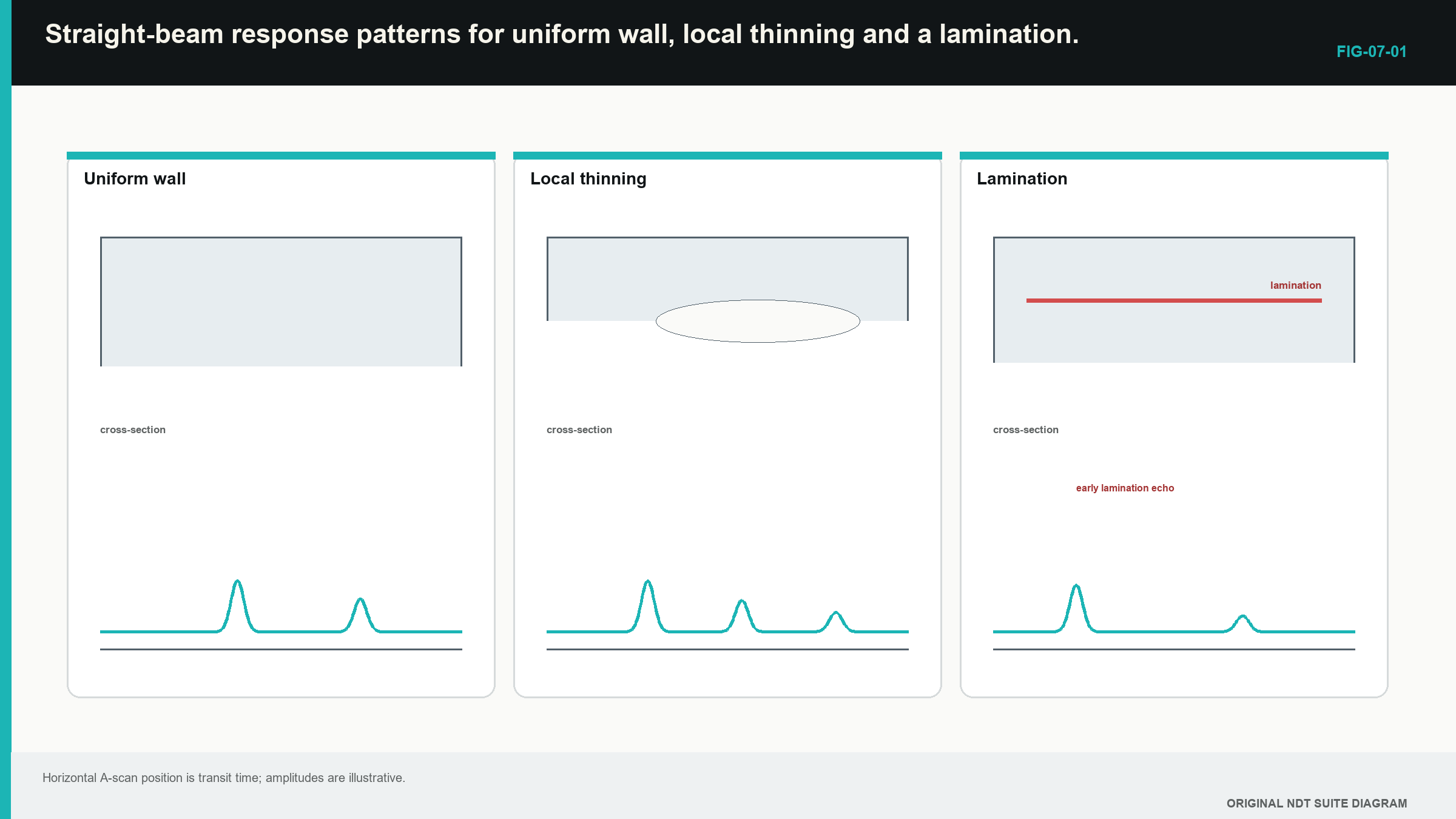
An early repeatable response is not automatically a lamination. Initial ringing, surface roughness, a coating boundary or component geometry can also create it. Identity becomes stronger when the response keeps a consistent depth over an area, changes at sensible edges and has a matching effect on the true back wall.

7.2 Three common timing arrangements

Single-echo timing measures from an established starting zero to one selected back-wall echo. It can work well when probe delay, coating and interface effects are corrected. It is vulnerable when the wrong echo enters the gate.

Multiple-echo timing uses the spacing between successive back-wall echoes. A fixed probe or coating delay can cancel because both peaks contain it. The method is valid only when the selected peaks come from the same pair of material boundaries.

Dual-element timing uses separate transmitting and receiving elements. Their sloping fields meet in the component. The total path forms a V rather than one normal line. As wall thickness changes, the intersection and path geometry change. The time-to-thickness relationship can therefore be nonlinear.

A dual probe is often useful for thin corroded wall because it reduces some initial-pulse interference. It has a shallow limit where the fields have not yet overlapped properly and a deeper region where they separate. Calibration must cover the intended thickness range. Extrapolating beyond that range can create bias.

Minimum measurable thickness is not one permanent number printed on the probe. It depends on pulse length, recovery, coating, surface, material and the instrument's measurement algorithm. A numeric display may continue producing values after the interface and back-wall pulses have overlapped too strongly for reliable separation.

Known steps through the intended range show where bias begins or repeatability collapses. The demonstrated lower bound is more useful than the smallest number the screen is willing to display.

7.3 Coatings, curvature and rough surfaces

A coating and the metal below it carry sound at different speeds. A simple single-echo reading can include travel through both materials. If the instrument treats all that time as steel time, the displayed number is not automatically the steel thickness.

The learner should first identify the measurement mode. A reading timed from the interface to one back-wall echo may include a fixed coating or probe delay. Echo-to-echo timing can sometimes avoid that fixed delay because it uses the gap between matching metal echoes. It works only when both selected peaks come from the same two metal boundaries. Regular-looking echoes from a lamination do not become back-wall echoes merely because the spacing is tidy.

Curved surfaces change the contact area. A probe on a small pipe can rock or point along a different path. A shaped shoe may improve contact, but that shoe becomes part of the test system. It must be included when the time response is checked on suitable known thicknesses.

Rough corrosion weakens and broadens the back-wall response. The strongest part of the echo may come from a pit shoulder rather than the deepest point. Scale, deposits and surface profile add more uncertainty to the acoustic contact. A stable low number is useful evidence, but the visible waveform must still support it.

A simple comparison helps. On a smooth known plate, remount the probe and observe the same back-wall pattern several times. Then place it on a rough region. If most echoes fall and the trace changes with rocking, coupling is part of the change. If one earlier wall response remains at a consistent position while the probe moves across a local area, real wall shape becomes more plausible.

Step up preview - separating several material layers

Several layers add their own travel times, and thin layers can produce overlapping echoes. Level 2 develops the full layer-time equation and the coating-bias calculation. Level 1 retains the practical rule: do not turn a mixed coating-and-metal time into metal thickness unless the selected mode has been demonstrated for that arrangement.

7.4 Mapping an area instead of one point

A point reading describes one acoustic footprint at one position. A corrosion map samples many positions. The physical wall between those positions is not directly measured.

Grid spacing controls the largest gap between measurement centres. Beam footprint controls the area contributing to each response. Pulse and echo-selection behaviour control the depth information. All three matter.

A narrow beam on a wide grid can pass between small pits. A broad beam on a fine grid can smooth a narrow pit with surrounding sound wall. Making the colour pixels smaller does not change either physical limit.

The next figure shows the combined problem. Notice that interpolation draws smooth colour between measured values. That surface is a visual model, not new measurements.

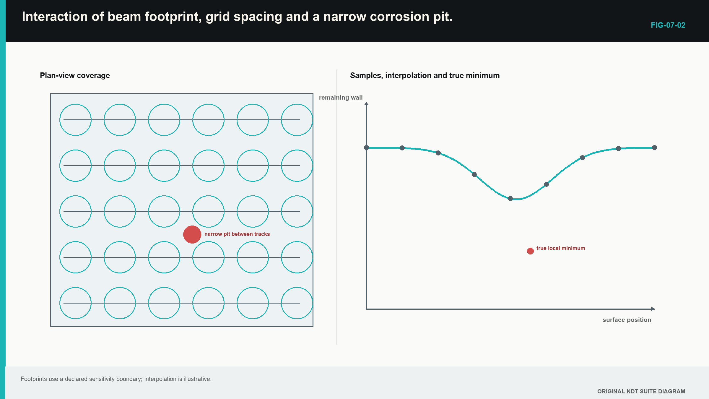
Missing and invalid readings should remain visibly missing. Filling them with normal thickness makes a map falsely healthy. Filling them with zero makes it falsely severe. A separate validity or coverage layer shows where defensible readings were obtained.

The phrase “minimum thickness” needs a defined area and sampling method. The minimum observed on a grid is not automatically the true minimum anywhere in the region.

For example, a technician may collect a valid 5 mm grid over most of a pipe elbow but lose coupling in one rough band. The correct map shows measured values over the valid region and an unmeasured band where the response failed. It does not interpolate healthy colour through the missing area. The report can state the minimum valid reading, the grid and footprint basis, and the incomplete coverage separately. This gives the decision-maker useful evidence without turning an acoustic blind spot into imaginary metal.

7.5 Checking velocity before trusting a number

The instrument turns travel time into thickness by using a sound velocity. That chosen value should suit the material, wave mode and temperature closely enough for the task. A steel value is not suitable for a polymer coating. A longitudinal-wave value is not suitable for a shear-wave path.

A known thickness gives the learner a direct check. Couple the complete probe system to a representative area with a known wall. Confirm the correct back-wall echo, then compare the displayed result with the known dimension. If the display is wrong by a similar proportion at several thicknesses, the velocity or distance scale may be wrong. If every value is shifted by about the same amount, the zero or fixed delay is more likely.

The known dimension must represent the same path that produced the echo. A calliper value taken beside a tapered region may not equal the acoustic path under the probe. Parallel surfaces are easier to use because the returning back-wall pattern is clear. A longer known path also makes a small timing error less dominant.

Successive back-wall echoes can help because their spacing represents another round trip through the same wall. That spacing can remove one fixed delay from the comparison. It does not remove a wrong material choice, temperature difference or mistaken echo identity.

For a first check, the learner records the material description, known thickness, selected velocity, probe arrangement and visible echo pair. That record makes the chosen value explainable. It is stronger than entering a familiar steel number and accepting the display because it has two decimal places.

Step up preview - uncertainty belongs to the whole measurement

Every thickness result is affected by more than the instrument resolution. Timing, zero, velocity, coating, surface condition, echo choice and probe position can all contribute. Repeated couplings reveal some placement variation, but they do not reveal one shared wrong velocity.

Level 2 develops practical uncertainty estimates, and Level 3 develops formal budgets and trend decisions. The two-unknown velocity-and-delay example moves to Level 2. No Level 1 assessment depends on that calculation.

7.6 Pit shape, footprint and response pattern

A narrow pit is not a flat back wall. Its curved surface has many local normals. Some sound returns from the shoulder while some is redirected away. If the footprint is larger than the pit, sound wall around it contributes to the received waveform.

General wall loss often keeps a broad back-wall response that moves earlier over an area. A local pit can produce a local time minimum, reduced amplitude and a broader or changing waveform. A lamination can create an early series and shadow the real wall. These patterns can overlap.

Probe movement is useful evidence. A broad thinning response should change smoothly. A pit response may pass through shoulders to a local minimum. Poor coupling often changes all echoes and improves after remounting. Adjacent A-scans provide context that one colour pixel cannot.

A smaller or focused field can improve localisation. It can also increase sensitivity to surface contact and stand-off. Representative pits are needed to establish how the chosen probe and scan pattern respond to the morphology of concern.

The reported value is an acoustic estimate over the sampled field. It is not a guarantee of the deepest physical point unless capability has been demonstrated for comparable pits, surfaces and sampling.

7.7 Step up preview - comparing surveys over time

Two surveys can be compared only when their positions and measurement arrangements are meaningfully aligned. The same grid spacing is not enough if the starting point moved. A different probe, temperature, velocity, gate rule or surface condition can also change the displayed minimum even when the component has not changed.

Level 2 develops registration and like-for-like survey comparison. Level 3 develops combined uncertainty and loss-rate decisions. Level 1 is not assessed on trend calculations. Its responsibility is to keep coordinates, settings, important A-scans, invalid regions and any equipment change so that a later comparison has honest evidence.

7.8 Valid, invalid and bounded results

A valid reading has a plausible and repeatable wall response inside the established measurement range. Its signal quality and path support the displayed number.

An invalid reading occurs when the instrument follows noise, an unresolved interface, an unintended path or a signal outside calibration. “No valid measurement” is more accurate than a convenient invented value.

A bounded result can still be useful. Evidence may show that wall lies below one reference step while the exact back-wall peak remains unresolved. The report can state that limit without pretending to know a precise thickness.

Automated maps should store a validity result with each number. Amplitude alone is not enough. A strong lamination echo can be stable while representing an internal boundary rather than total wall. Echo spacing, waveform similarity, neighbour continuity and back-wall plausibility can all help.

A thickness statement should identify its claim:

• thickness at one stated point;
• minimum valid thickness observed on a defined grid;
• estimate of minimum wall over a defined area with demonstrated sampling capability.

Those statements use the same unit but claim different amounts of knowledge.

The straight-beam and thickness foundation in this chapter follows the cited international ultrasonic training reference. [R001]

In plain words

• Thickness arithmetic is simple only after the correct back-wall echo is identified.
• Uniform wall, thinning and laminations create different patterns across several traces.
• Single-echo, multiple-echo and dual-element modes use different timing models.
• Coating time cannot be treated as metal time without correction.
• Grid spacing and beam footprint together control area sampling.
• A colour map interpolates between measurements and can hide missing data.
• Velocity, zero, temperature and position records affect later comparison between surveys.
• A valid “no reading” is better than a precise number from the wrong echo.

Key terms

• Back wall: far surface used for the wall echo.
• Lamination: internal planar separation or elongated discontinuity.
• Footprint: region contributing to a probe response.
• Grid: planned measurement positions.
• Registration: alignment of coordinates between datasets.
• Bounded result: evidence that limits a value without claiming an exact measurement.

Key relationships

• d = ct/2: simple one-layer pulse-echo thickness after correct time and velocity are established.
• A coating and the metal below it can add different travel-time contributions.
• Successive back-wall spacing can reduce a fixed-delay effect when the same boundaries produce both echoes.

Common mix-ups

• The first stable echo is not automatically the far wall.
• Echo-to-echo mode does not prove correct peak selection.
• Minimum observed grid value is not automatically true area minimum.
• More pixels do not create a smaller beam footprint.
• Missing readings should not be silently replaced by normal wall or zero.

Bridge to Chapter 8

Straight-beam work uses a mainly normal path. Welds and planar targets often need sound to enter at an angle. Chapter 8 introduces the probe index, refracted angle, sound path, first and second legs, skip distance and the evidence needed to connect one angle-beam response to component geometry.

Sources and further study

• [R001]