Building a PAUT Coverage Story from the Component

Why this matters

Coverage is not the coloured area inside a sector fan. It is a supported statement about which component volume was examined for which target conditions, from which probe positions and within which demonstrated limits. This chapter develops that statement using one weld cross-section. The drawing begins with the component and credible discontinuity orientations. It then gains the scanning surface, probe and wedge, beam regions, electronic laws and mechanical movement. At every stage, access and evidence decide what can honestly be claimed.

What you already need

• A focal law creates one finite beam condition rather than a single line.
• Law groups can change aperture position, angle or focus.
• Encoded scanning attaches complete law groups to component position.
• Calibration and performance checks establish particular relationships.
• Reflector orientation, material and geometry affect response.

What you will learn

• Begin technique design with component, material, target and required information.
• Add probe positions and beam regions to an evolving weld cross-section.
• Connect access, coupling and scanner footprint to achievable coverage.
• Use a simple ray projection as a planning check without calling it proof.
• Distinguish geometric intersection, demonstrated response and validated capability.
• State clearly when conditions fall outside the demonstrated technique.

Words you will meet

• Examination volume: the defined material region intended to be examined.
• Target population: the discontinuity types, locations and orientations the technique is meant to address.
• Coverage: supported interrogation of the defined volume under stated conditions.
• Shadow zone: a region where geometry or another interface prevents useful interrogation.
• Complementary direction: another beam or probe direction that adds different sensitivity.
• Demonstration: observed evidence from known features using the proposed configuration.
• Essential variable: a technique property whose change can affect supported capability.

35.1 Stage 1: draw the real examination object

Begin with a cross-section of the component at a useful scale. For a weld, show thickness, bevel or preparation, root, cap, counterbores, mismatch, reinforcement and nearby surfaces that can reflect sound. Use controlled drawings and compare them with the as-built item.

Define the examination volume. It may include the weld, heat-affected regions and a stated width of adjacent parent material. Mark the scanning surfaces and the physical regions that cannot be reached. Add a component datum and coordinate directions so later probe positions and indications have one reference.

The material is part of the object, so record product form, heat treatment and structure where they affect sound. Rolled plate, forging, casting and weld metal can attenuate or scatter differently. Curvature and temperature can change coupling and beam entry.

At this first stage, do not draw a probe. The component should be understandable before any equipment is chosen. Starting with a favourite array encourages the design to solve the probe's capabilities rather than the inspection problem.

35.2 Stage 2: add credible target conditions

A target population is a reasoned list of the conditions the examination is intended to address, including likely zone, depth, orientation, surface connection and acoustic behaviour. The list guides beam direction and demonstration; it does not claim the component contains every listed condition.

For a fusion weld, credible targets can include lack of fusion along a fusion face, root-related conditions, cracks with process-dependent directions, inclusions and volumetric zones. Normal geometry can produce competing responses at the cap, root, counterbore or backing. The actual joining process matters. Flux slag is not a sensible default for every gas-shielded process, while oxide, tungsten or other inclusions have different process links.

For wrought products, material flow can align inclusions or structure. Rolled-plate laminations often lie broadly parallel to the surface. For cast products, coarse grains and shrinkage or porosity can produce strong scattered response. Service damage such as fatigue or stress-corrosion cracking can branch and orient with stress rather than fabrication geometry.

On the cross-section, draw representative target planes or zones rather than generic flaw icons. Mark which directions are likely to meet each target favourably. A planar reflector may need more than one direction because specular reflection can send energy away from the probe.

35.3 Stage 3: state the information required

Different decisions need different evidence. Detection asks whether a relevant response can be found. Location asks where it lies. Characterisation asks what physical explanation best fits. Sizing asks for a supported dimension. Evaluation compares the established information with the applicable criteria.

A technique demonstrated only for detection should not be assumed to size height. A strong artificial-target response does not by itself establish natural-flaw reliability. The design should name the required output before choosing settings.

The governing inspection and product documents supply scope, technique constraints and acceptance requirements. They have different roles. A PAUT method document may describe examination without supplying product acceptability. A syllabus can identify learning topics without granting work authority. [R042] [R060]

For this study chapter, keep the technical question practical: the setup must gather enough valid ultrasonic and positional evidence for the defined Level 2 analysis task. Formal authorisation and reliability claims are moved to later chapters.

35.4 Stage 4: choose candidate wave directions and frequency

Add possible sound paths to the cross-section. Select wave mode and direction from target orientation, component geometry and accessible surface. Mark direct and reflected paths that could provide useful interactions. Also mark surfaces that can create strong geometric echoes or shadowed regions.

Frequency balances resolution and penetration. Higher frequency gives shorter wavelength in the same material and can support finer separation. It is usually more affected by attenuation and scattering. Lower frequency can improve penetration and response stability while reducing separation of nearby echoes.

Bandwidth and pulse length also matter. A broad useful band can support a shorter pulse and better axial separation, but nominal centre frequency alone does not describe it. Probe damping, wedge, filters, digitisation and the component shape the received pulse.

Compare candidate arrangements on representative paths. Observe signal-to-noise behaviour, pulse separation and target response. Do not select a probe only because its nominal frequency worked on another material or thickness.

35.5 Stage 5: place the array, aperture and wedge

Now add the physical probe and wedge to the scanning surface. Check the complete footprint, not only the nominal exit point. Include room for the scanner, encoder wheel, cable bend, couplant delivery and start or stop overrun.

Choose the array arrangement for the required plane of control. A linear array suits many weld sectors and electronic aperture steps. A matrix may add second-plane control but also adds channel, setup and evidence demands. A specialised curved array can improve contact for one geometry.

Choose a physical aperture that provides useful sensitivity and beam width while leaving sufficient steering and electronic-step room. A larger aperture is not automatically better. It can enlarge the footprint, reduce end positions, change focus and make contact or steering more demanding.

Select a wedge or delay arrangement that fits the component and supports the intended refracted directions. A flat wedge rocking on a curved surface is a coupling and geometry problem even when the software draws a stable fan. Wedge wear, velocity, angle and element reference remain law inputs.

On the evolving cross-section, draw first, middle and last aperture positions when electronic stepping is used. Show the associated wedge references. This reveals whether the virtual positions actually fit inside the physical probe and scanning access.

35.6 Stage 6: replace centre lines with useful beam regions

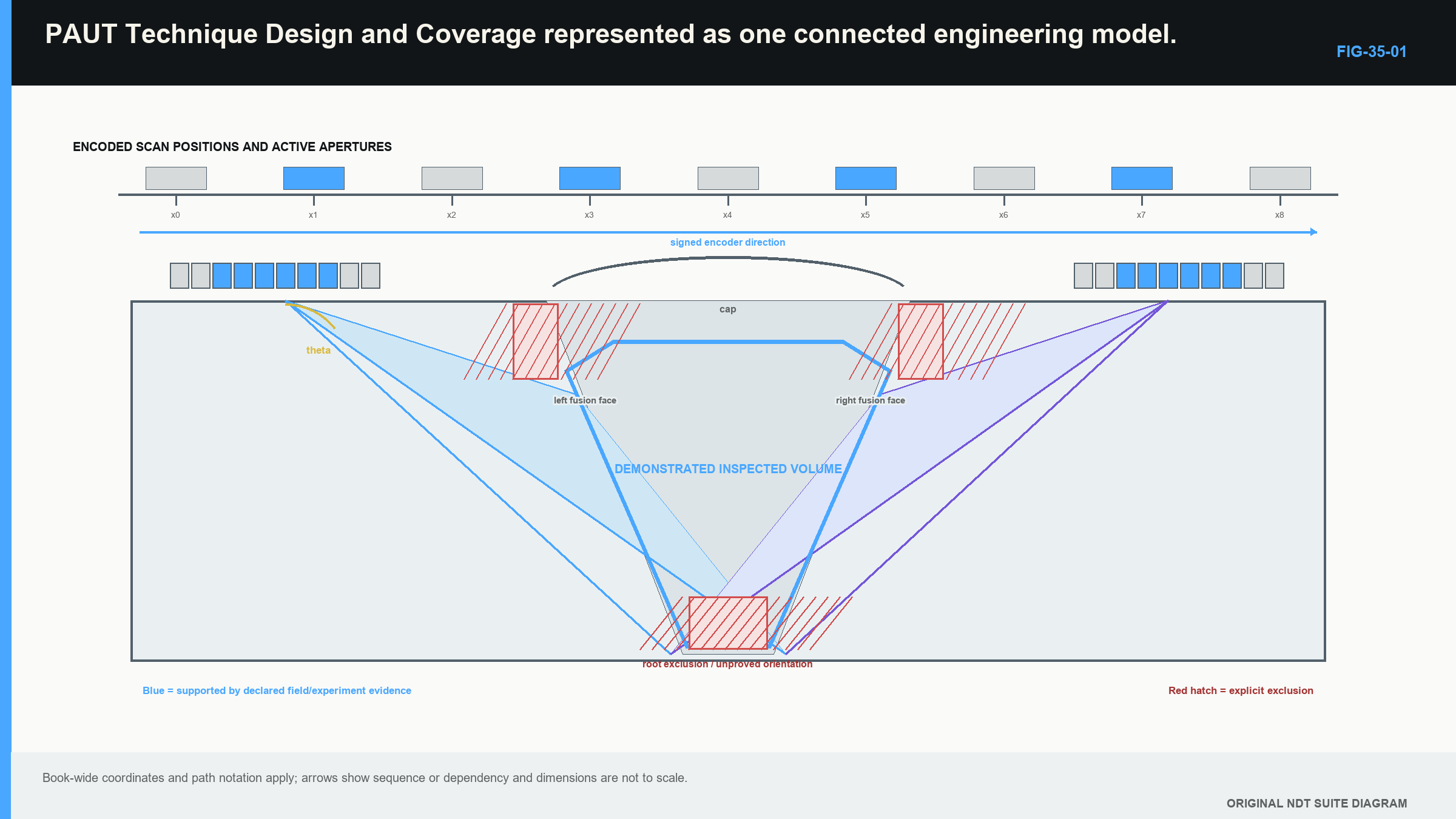
Centre lines help check whether a nominal path can reach a target, but they do not show beam width, focal region or off-axis response. Around each important centreline, add the beam region supported by calculation, characterisation or reference-target evidence.

Check near-surface, mid-wall and far-surface regions. Include the fusion faces, root, cap and transitions where applicable. Look for gaps between useful beam regions, not only gaps between ray lines. Consider whether extreme laws remain inside the calibrated and demonstrated range.

Add more than one direction when the target population needs orientation diversity. A beam from the opposite side or a changed skew can provide a complementary interaction. Several nearly identical angles from the same aperture may add little independent sensitivity.

Also mark side-lobe or mode-converted paths that could produce competing responses. Coverage design includes the ability to interpret the evidence, not only to deliver energy somewhere in the component.

The following figure shows the cross-section after these layers have been added. The shaded volume represents demonstrated useful support, while dashed regions remain uncertain or inaccessible. [R016]

35.7 Stage 7: add mechanical movement and encoded spacing

Electronic laws cover only the region available from the current physical probe location, so add the planned mechanical path, scan limits, index offsets and complementary passes. Include approach and exit distances needed to cover the boundaries.

For a one-line encoded weld pass, show the probe offset from the weld centreline and the beginning and end coordinates. For a raster, show each line and the index spacing. Overlap is the shared verified useful coverage between neighbouring passes, not merely the distance between their centre lines.

Select acquisition increment and travel speed within the demonstrated data and scanner capability. Fine spacing does not repair a weak beam. Coarse spacing can miss short response changes or distort measured length. The complete law set must be stored at every required position.

Mark obstacles, attachments and surface damage. Plan controlled overlap and supplementary passes around interruptions. If a region remains inaccessible, keep it visible in the coverage drawing and later report. Empty space in the plan should not be filled with optimism or decorative fan lines.

35.8 A simple projection is a planning check

For a straight ray in a planar isotropic region, a nominal refracted angle can be projected from depth to a surface distance. The physical meaning comes first: the tangent connects the vertical depth and horizontal offset of the central path.

35.9 Stage 8: demonstrate the proposed arrangement

Use known features or a suitable representative specimen with the complete field configuration. Include probe, wedge, couplant, scanner, law groups, acquisition settings and analysis presentation. Challenge the edges of the proposed range, not only its easiest central point.

Observe whether target responses are detectable and correctly located across relevant angles, depths and probe positions. Check coupling and data continuity. Compare first and last apertures, sector edges, near and far regions and any transition between focus or mechanical passes.

Separate three levels of evidence:

• Geometric intersection: a nominal path crosses the target region on a drawing.
• Demonstrated response: a stated known target responds under stated trial conditions.
• Capability claim: evidence supports the defined target population and range to the required level.

Geometric intersection helps planning; demonstrated response supports the tested configuration; a capability claim may need broader validation, reliability evidence and authorisation. Do not promote one successful open demonstration into a universal probability-of-detection claim.

Record limitations as technical results. A shadowed root sector, weak extreme angle or inaccessible band is not a paperwork inconvenience. It defines where the technique's evidence ends.

Read one finished coverage drawing from left to right

Start at the component datum and follow the first probe position. Confirm that the wedge footprint fits the prepared surface and that the scanner can reach the planned start. Follow the lowest useful law into the near-side region and note which target orientation it supports. Then follow the middle and highest useful laws through the weld and toward the far-side boundary.

Move to the first electronic aperture and compare it with the last. Their nominal angles may be the same while their entry points and edge performance differ. Check whether each remains inside the calibrated law range and whether its useful beam region reaches the intended boundary.

Next, follow the mechanical path. At the beginning and end of travel, decide whether the probe can overrun far enough to place the whole beam region over the examination volume. At each obstacle, mark the affected coordinates and the supplementary or overlapping pass. At every index move, compare verified coverage width with line spacing.

Now examine the target list rather than the shaded volume. For each credible target orientation, identify at least one supported interaction. A shaded point crossed only by an unfavourable centreline may not have useful sensitivity. A region reached by several nearly identical beams may have less orientation diversity than its colour suggests.

Finally, inspect the exclusions. Name the near-surface zone, geometric shadow, weak angle, poor-coupling band or inaccessible strip that limits the claim. If another direction or method addresses it, link that evidence without pretending it came from the original pass.

This left-to-right review turns a coverage drawing into a technical story another reader can challenge. It also keeps the claim tied to physical probe positions rather than to the size of the software fan.

Repeat the reading from the opposite end of the component. This reverse review often exposes an assumed overrun, a sign error or a far boundary reached only by the central ray. It also shows whether a complementary direction genuinely adds target sensitivity or merely repeats the same path from a nearby position.

Attach observed evidence to the drawing at representative locations. A small note can link a reference response, encoded trial or coupling observation to the law and position that support the shaded region. The drawing then becomes an index to evidence rather than an illustration detached from the dataset.

Keep uncertainty visible through boundaries and words. Solid shading can represent demonstrated support, lighter shading a modelled candidate region, and an outline an inaccessible or unresolved zone. The legend must state the convention. Visual certainty should not exceed technical certainty.

Update the cross-section when the actual component differs. A revised local thickness, counterbore or reinforcement profile can change both useful and competing paths. Keeping the nominal drawing while correcting only the screen geometry breaks the link between the coverage claim and its evidence.

Give the coverage statement a version tied to that drawing and law set. If either changes, the old shaded volume remains historical evidence rather than a reusable promise. This simple link prevents a later setup with a familiar name from inheriting coverage it has not demonstrated.

35.10 When the real component differs

Field conditions can move outside the demonstrated range. Material may be noisier, surface curvature greater, access narrower or wedge temperature different. The correct technical response is to identify the changed condition and its effect on beam path, coupling, data or interpretation.

Do not quietly increase gain and keep the original coverage claim. Gain can improve display height while noise and beam suitability remain unchanged. Do not rename a setup file to make a new geometry appear approved.

At Level 2, stop the unsupported extension, preserve the observations and use the controlled technical route for review, changed technique or complementary examination. The important learning point is the evidence boundary: successful performance inside stated conditions does not automatically transfer outside them.

Step up: formal validation and change control

Later chapters turn the coverage story into validation variables, approval evidence and change-control decisions. They address representative specimens, model assumptions, blind trials, essential variables and reliability. Those governance and qualification topics are not assessment dependencies in this crossover chapter.

In plain words

• Technique design starts with the component and target population, not the probe catalogue.
• Coverage is tied to a defined volume, target conditions and evidence range.
• Target orientation influences which beam directions are useful.
• Physical access, wedge fit and scanner footprint can limit an otherwise possible path.
• Central rays help planning but do not show the complete acoustic field.
• Electronic laws and mechanical movement must be considered together.
• A demonstrated target response is bounded to its stated configuration and conditions.
• Regions outside the evidence remain limitations until addressed.

Key terms

Examination volume; target population; coverage; scanning surface; shadow zone; complementary direction; demonstration; evidence boundary; essential variable.

Key relationships

• component + material + target orientation -> candidate wave directions;
• frequency + aperture + wedge + path -> usable beam response;
• electronic beam regions + mechanical paths -> planned volume coverage;
• nominal ray intersection < demonstrated target response < supported capability claim;
• changed field condition -> review of which coverage evidence still applies.

Common mix-ups

• A coloured sector fan is not a coverage statement.
• Central-ray density is not acoustic overlap.
• Reference-target detection is not universal natural-flaw reliability.
• More gain is not a substitute for access, direction or signal-to-noise ratio.
• “Not demonstrated” is not the same as “proved impossible,” but it cannot be reported as covered.

Bridge to Chapter 36

Chapter 36 begins after valid coverage and data quality have been established. It follows three practical response cases, then turns the observations into a restrained sequence of interpretation, sizing, comparison with supplied criteria and reporting.

Sources and further study

• [R016]
• [R042]
• [R060]