When the Simple Material Model Fails

Why this matters

A law that is accurate in isotropic carbon steel places a response inside an austenitic weld, yet the image changes when the probe scans from the opposite side. The display may still look precise while the beam energy follows a different path. Complex material and geometry problems should begin with a practical diagnostic sequence: state the simple assumption, identify what physical behaviour can break it, observe the symptom and select the next evidence or model. This chapter applies that sequence to textured welds, coarse grains, composites, cladding, curved components and additive manufacture without assuming prior study of elasticity tensors or numerical wave modelling.

What you already need

• Competent PAUT Level 2 knowledge of wave modes, refraction, focusing and displays.
• The distinction between a focal law, a propagation path and a reconstructed coordinate.
• Practical awareness of attenuation, scattering, noise and mode conversion.
• The qualification evidence layers from Chapter 42.
• Basic use of velocity, time and distance in a pulse-echo path.

What you will learn

• Recognise when one isotropic velocity is no longer an adequate model.
• Link common complex materials to visible PAUT symptoms and failure mechanisms.
• Choose a model hierarchy that grows only as the decision requires.
• Separate material, target, geometry and processing effects.
• Validate corrections with independent observables and cases.
• State a defensible boundary when prediction remains uncertain.

Words you will meet

• Isotropic: having the same relevant properties in every direction.
• Anisotropic: having properties that depend on direction.
• Inhomogeneous: changing in property from one position to another.
• Phase direction: direction associated with the advancing phase front.
• Group direction: direction in which wave energy travels.
• Quasi-mode: wave mode whose motion is not purely longitudinal or shear.
• Structural noise: response caused by material structure rather than a target.
• Homogenisation: replacing fine structure with an effective bulk model.
• Stochastic model: model representing variable structure through distributions.
• Model form: chosen physical structure and assumptions of a model.

43.1 Begin with the assumption that produced the screen

Most familiar PAUT laws treat each region as homogeneous and isotropic. One longitudinal velocity and one shear-wave velocity describe travel time and refraction. In wrought ferritic products this approximation is often useful. The first diagnostic step in an unusual component is to write that assumption beside the displayed result.

The assumption can fail in two different ways. An anisotropic material changes wave behaviour with direction. An inhomogeneous material changes from place to place. An austenitic weld can be both because elongated grains have directional properties and their orientation changes across weld zones.

When direction matters, the normal to a constant-phase surface and the direction carrying acoustic energy may differ. The screen can therefore reconstruct along the nominal phase or ray direction while the strongest energy travels elsewhere. Particle motion also need not be purely parallel or perpendicular to propagation, so the modes are described as quasi-longitudinal and quasi-shear. [R006]

The practical consequence is larger than travel-time error. Refraction angle, beam skew, focal position, beam width, polarisation, attenuation and scattering may all change. Moving a displayed cursor after the event corrects only a coordinate. It does not restore field support that never reached the target.

The following figure separates the nominal model from the energy path and geometric complication.

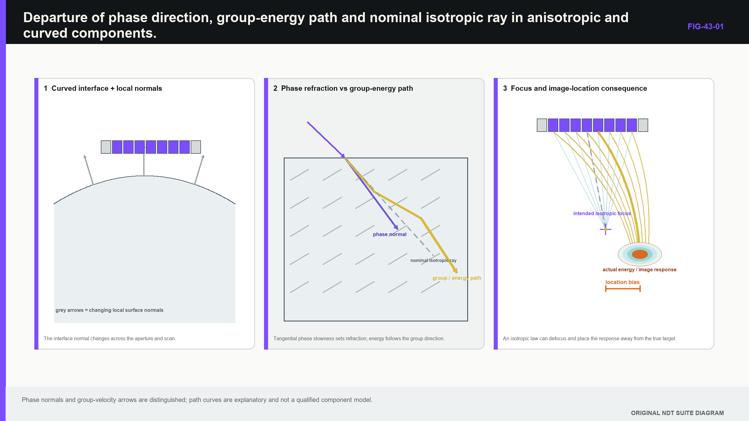
Notice that an apparently small time correction does not prove the energy direction, focus or target response.

43.2 Use one diagnostic pattern for every complex component

The Level 3 diagnostic can be written as four lines. First state the simple assumption. Second name the physical behaviour that can break it. Third identify the screen or scan symptom expected from that failure. Fourth select the next observation, experiment or model that can separate competing explanations.

For example, the simple assumption may be a constant isotropic shear velocity. Textured weld metal can break it by changing speed and energy direction with orientation. Screen symptoms may include opposite-side asymmetry, shifted peaks, broadened focus and unstable amplitude. The next evidence may be travel-time mapping, beam-skew measurement, lower-frequency comparison and representative targets from both directions.

This pattern prevents premature model escalation. A strange response can also come from wrong geometry, coupling loss, faulty elements, a law identity error or processing. Check those simpler causes before attributing every untidy image to exotic material physics. Complex materials are real; they are also a dangerously convenient alibi for ordinary setup mistakes.

Useful observables include arrival time, response movement with probe position, angle of peak response, waveform stability, beam width, opposite-side behaviour, target-free noise distribution and relationship to known boundaries. Record the raw data and processing state so that a display setting does not become confused with a material effect.

43.3 Follow an austenitic weld from texture to symptom

Austenitic weld metal often develops elongated grains along solidification directions. Velocity and attenuation can depend on propagation direction and polarisation, while coarse oriented structure can scatter energy. [R008] A nominally focused beam may skew, split or broaden. Structural echoes can resemble flaws and genuine target responses can fall into grain noise.

The continuing case is a dissimilar-metal weld containing ferritic parent, buttering, austenitic weld metal and cladding. A simple model assigns one velocity to each ideal planar region. The real component adds uncertain interfaces, changing grain direction and local curvature. The law is therefore a hypothesis about a path rather than proof that the path exists as drawn.

The first scan direction gives a strong planar response near one fusion boundary. The opposite direction gives weaker, broader energy at a shifted coordinate. This is not automatically a contradiction. The two paths encounter different texture and may favour different target orientations. The stronger image is not automatically the correct one.

Next evidence should challenge both path and target explanations. Measure known-reflector arrival times across relevant directions. Scan a small reflector to estimate beam skew and width. Compare opposite-side responses for targets with established position. Record target-free structural noise. If lower frequency is considered, test whether penetration and stability improve without losing required resolution and orientation support.

Low-frequency arrays have shown useful penetration in some coarse cast and weld applications, but their result remains tied to probe construction, aperture, scan increment and material. [R011] Frequency change is a design substitution that needs application evidence, not a universal cure for a difficult weld.

43.4 Treat coarse-grain noise as a population

When grain scale becomes significant relative to wavelength, scattering raises structural noise and disturbs phase. Moving the probe a small distance changes the set of grains contributing to the waveform. The resulting background is not one fixed trace; it is a population varying with position, path, aperture and frequency.

The simple assumption is that repeat scans through the same nominal material produce a stable coherent field plus small random noise. What breaks is the interaction between wavelength and local microstructure. Screen symptoms include speckle that reorganises with position, unstable amplitude, broadened responses and loss of coherent summation.

Measured sound fields in cast austenitic stainless steel demonstrate strong microstructure effects on propagation and penetration. [R012] Simulation work also shows that actual-grain and synthetic statistical models can produce different echo amplitudes. [R013] One measured patch or one random simulated microstructure cannot represent the whole component population.

Characterise target-free regions representative of the inspection volume. State whether noise is measured as root-mean-square (RMS) waveform level, envelope distribution, maximum image pixel or another metric. Preserve bandwidth, aperture, gate and processing definition. A maximum-pixel-to-average-background ratio cannot be compared directly with an RMS A-scan SNR unless the definitions are reconciled.

Averaging, larger apertures or coherent processing may improve stability in some cases. They can also suppress local responses, mix changing material paths or fail when phase is already decorrelated. Test target and non-target populations, not only whether the background image becomes prettier.

43.5 Decide whether a laminate can be treated as one medium

Composite laminates contain directional fibres, layers and interfaces. Fibre direction changes velocity and attenuation. Layer boundaries create repeated reflections, and defects such as delamination can be extended and highly directional. Curved structures add thickness and orientation change. Wavelength, architecture, geometry and defect type all influence penetration and image response. [R003]

The simple assumption is an effective homogeneous medium. It can be useful when wavelength is large relative to ply scale and the required observable is insensitive to individual layers. It begins to fail at higher frequency, oblique incidence or when interlayer response matters. Symptoms include path-dependent travel time, repeated interface bands, mode complexity and strong orientation dependence.

The next model may explicitly represent layer velocities and thicknesses, or it may retain an effective model with a larger validated uncertainty. The choice depends on the decision. A gross delamination screen may need less layer detail than accurate depth through a highly anisotropic lay-up.

Validate homogenisation against measured times and field or target response over relevant angles, orientations and thicknesses. A fit at normal incidence is not proof at the oblique paths used in PAUT. Bonded structures also require precise condition language. A void, weak adhesive layer and kissing bond need not produce the same response. “Bond integrity” is too broad when the evidence supports only one defined condition.

43.6 Separate cladding effects from deeper weld behaviour

Cladding and overlay affect the beam before it reaches the base material. Surface condition changes coupling. Thickness and texture alter delay, refraction and attenuation. The bond interface can generate coherent echoes and mode conversion. A law generated for an unclad component can be wrong even if the deeper base-metal velocity is correct.

The visible symptom may be near-surface clutter, a shifted deeper response, angle-dependent loss or a multi-leg feature from the overlay interface. Time gates and image masks can reduce clutter, but they can also hide evidence. The raw signal should remain recoverable and the suppression range should be qualified.

Measure or map cladding thickness where its variation can matter. Compare unclad and representative clad paths where possible. Check timing, angle and target response, not only amplitude standardisation. If variation exceeds the supported correction range, partition the component, use local calibration or limit the qualified region.

A single empirical delay correction may improve one reflector while leaving path direction and beam shape wrong. The next evidence should include more than the calibration target used to derive the correction. Hold-out positions and orientations are required to show that the correction transfers within the stated region.

43.7 Let local surface normal drive curved-component reasoning

Curvature changes the surface normal beneath each part of the wedge. A flat wedge can rock, lose contact and place its exit point differently from a planar model. Arc length, chord, developed distance and component coordinate are not interchangeable.

The simple assumption is a two-dimensional section with constant surface orientation. Nozzle intersections and blend regions break it through changing curvature, thickness transition and out-of-plane geometry. Symptoms include response drift along the scan, asymmetric coupling, misplaced boundaries and apparent coverage in a 2D view that disappears in three dimensions.

Begin with measured or controlled surface geometry and registration. Evaluate wedge contact across the footprint. Use a three-dimensional path or field model when the claimed volume changes out of plane. Confirm critical boundaries with representative targets or known geometry features. A 2D sector cannot prove a volume that is not invariant along the scan.

Thick sections add attenuation, beam spread and long receive time. A large aperture can improve nominal focusing while spanning more material variation and contact error. Separate near- and far-region groups may be more robust than one compromise focus. The longer receive window also feeds back into automation rate and completeness from Chapter 40.

43.8 Define the additive component population narrowly

Additive manufacture can produce directional texture, porosity, lack-of-fusion populations, rough surfaces and complex near-net geometry. Build direction, scan strategy, material, heat treatment and surface finish influence both expected discontinuities and propagation. “Additive component” is therefore not a defensible single population.

The simple transferred assumption is that a wrought-material setup applies because the alloy name and nominal velocity are similar. Directional texture or heterogeneous porosity can break that assumption. Screen symptoms may include orientation-dependent amplitude, structural noise, shadowing, shifted paths and expected reflections from internal channels or lattices.

A digital design model helps predict geometry paths, but the as-built component can differ. Registration error between design and component may create systematic artefacts that resemble propagation failure. Establish the as-built surface and relevant internal geometry tolerance before tuning material parameters to make the image fit.

Qualification identifies the represented process, machine or process family, alloy, build orientation, heat treatment, surface condition, thickness and target morphology. Transfer beyond them requires an evidence argument. Narrow populations are not an inconvenience here; they are how a highly variable manufacturing route becomes testable.

43.9 Grow the model hierarchy one decision at a time

Start with the least complicated model that can answer the decision. The sequence may move from isotropic rays to piecewise isotropic regions, curved interfaces, anisotropic ray or group paths, deterministic full-wave models and stochastic ensembles. Each step introduces new inputs and new ways to be confidently wrong.

An anisotropic model needs material axes, elastic constants or a validated reduced description, and coordinate transforms. A heterogeneous weld model needs zone geometry. A layered model needs thickness and interface properties. A stochastic model needs distributions, spatial statistics and enough realisations to describe variation.

Do not add a parameter merely because software exposes it. Identify the observable it changes and the evidence that bounds it. Grain orientation adjusted until one target becomes bright is calibration, not independent validation. If several parameter combinations reproduce the same arrival time, the model may be unidentifiable for amplitude or field prediction.

Compare a small model hierarchy on common raw data and metrics. If isotropic, piecewise and anisotropic models locate a boundary similarly while predicting different amplitudes, model-form uncertainty may be modest for location but large for sensitivity. If path identity and coordinates diverge, the uncertainty is structural and should remain visible.

Model selection should use independent observables such as arrival time, measured beam skew and opposite-side behaviour. Selecting the reconstruction that produces the brightest indication biases the conclusion toward concentration rather than physical credibility. [R006] [R008] [R012] [R013]

43.10 Measure direction, attenuation and field behaviour deliberately

One velocity measured in one direction does not characterise an anisotropic region. A useful programme samples directions and polarisations related to the intended paths, with specimen orientation tied to a material frame. Sparse measurements can support a reduced model, but interpolation between them remains an assumption.

Attenuation measurements combine coupling, beam spread, scattering and absorption unless the experiment separates them. Through-transmission pairs, several path lengths or comparative reference paths can help. Retain direction, frequency band, aperture and measurement method. One decibel-per-length number does not describe every route through a textured weld.

Beam skew and focal degradation can be observed by mapping a field or scanning a small reflector through representative material. Displacement from the isotropic prediction indicates group-path change. Broadening or splitting indicates coherence loss. Repeating at different positions separates systematic texture from stochastic variation.

Correcting the nominal path to a measured peak may improve the displayed coordinate. It still does not prove that targets on either side of the corrected centre receive adequate energy. Field width, orientation support and position-to-position stability should therefore accompany the peak correction.

43.11 Use the velocity-ratio equation only inside its assumptions

Before introducing anisotropic direction changes, consider the simplest visible error. A direct pulse-echo path is interpreted with a velocity higher than the actual effective group speed. The measured time is correct, so the displayed distance becomes too large in the same ratio as the model velocity.

The equation is dimensionally consistent because each side is a ratio. It can explain a first screening result, but should not be promoted into an anisotropic field solution.

The failure case occurs when the same apparent bias changes with scan direction or reflector position. A single ratio can no longer describe the component. Measure direction and path behaviour, then adopt a piecewise, anisotropic or empirical model with an explicit range.

43.12 Validate observables, not image attractiveness

Validation should compare the quantities used by the technique: arrival time, beam direction, focal position, field width, SNR, target response and artefact behaviour. Agreement in one does not guarantee agreement in another. A model can predict time accurately while missing amplitude because it omits attenuation and scattering.

Use evidence independent of model calibration. If velocity or grain orientation is fitted to one target, test different targets, paths or specimens. Hold-out evidence is especially important when several parameters can compensate for one another.

Signal processing may improve visibility in coarse welds, but it can also alter morphology, phase and amplitude. Raw traceability and target-based validation are essential. [R062] Processing parameters and software identity belong to the qualified inspection system rather than being treated as harmless display preferences.

Development and confirmation regions should be separate when processing is tuned to structural noise. A filter that suppresses one grain pattern can fail elsewhere. Compare raw and processed target and non-target data to show whether the intended signal is preserved and whether false-call behaviour changes.

When no available model predicts the component well enough, representative empirical demonstration may carry more of the claim. The correct response is usually a narrower range and stronger retained evidence, not an elaborate unvalidated image.

43.13 Control empirical corrections and complementary evidence

An empirical travel-time or sensitivity correction can be useful when a full material model is unavailable. Record support coordinates, directions, target types, frequency, temperature, interpolation method and residuals. Encode the valid range so software cannot apply the correction silently beyond its evidence.

The correction should retain residual uncertainty. If residuals are discontinuous or depend strongly on path, divide the component into regions or redesign the technique. Extrapolation outside support points is a new claim, even when the resulting image looks smooth. [R006] [R008] [R011] [R012] [R062]

Complementary evidence should challenge a particular uncertainty. Lower frequency tests penetration and phase stability. Opposite-side insonification tests direction dependence. A movable conventional probe tests local orientation response. Material mapping tests the propagation hypothesis. Surface metrology tests registration and curvature.

Agreement is not independent when all methods use the same wrong geometry or coordinate model. Register each result in a common frame and retain its own assumptions. Partitioned techniques also need overlap evidence at regional boundaries so that the solution does not create an unexamined seam.

43.14 State the model boundary in the released claim

Return to the dissimilar-metal weld. Directional time measurements, field mapping and representative targets support one model and frequency over declared zones and scan directions. Structural-noise data define an analysis range. Opposite-side evidence remains asymmetric but predictable inside those zones.

The release can claim the demonstrated target and component population. It cannot export the correction to another weld by nominal alloy or process similarity alone. If material characterisation does not support a stable propagation model, the technique can remain useful through representative empirical evidence, but transfer becomes correspondingly narrow. [R008] [R012]

The report identifies material axes, zone geometry, property sources, fitted parameters, residuals, model version and raw validation cases. Future sectioning or material evidence can then revise the interpretation without erasing the original reasoning.

In plain words

• A precise PAUT image can still be based on the wrong material or geometry model.
• Anisotropy changes behaviour with direction; inhomogeneity changes it with position.
• Energy direction can differ from the nominal phase or ray direction.
• Every complex case should link assumption, failure, visible symptom and next evidence.
• Noise in coarse material is a population, not one background trace.
• More complex models need more measured or bounded inputs.
• Correcting a cursor does not restore missing beam support.
• When prediction remains weak, narrow the claim and strengthen empirical evidence.

Formal synthesis

Complex PAUT applications challenge the homogeneous isotropic approximation through directional elasticity, spatial variation, scattering, layering, curvature and registration. Diagnosis begins with the simplest model and a physical prediction of its failure symptoms. Model complexity grows only where a stated decision requires it, with independent measurements of time, direction, field, noise and target behaviour. Direct-path velocity scaling remains useful within strict assumptions but cannot represent path change. Empirical corrections and complementary views retain bounded support, residual uncertainty and dependency. The released technique states the material-model boundary as part of its performance claim.

Key terms

• Anisotropy: directional dependence of acoustic behaviour.
• Inhomogeneity: spatial variation of material behaviour.
• Group direction: direction of acoustic energy travel.
• Structural noise: material-structure response competing with targets.
• Homogenisation: effective replacement of fine structure by a bulk model.
• Model-form uncertainty: uncertainty caused by the chosen physical model itself.
• Empirical correction: measured adjustment valid only within its support range.

Key relationships

• EQ-43-01 links velocity ratio to distance ratio only for the stated direct path.
• Arrival-time agreement does not prove field shape, amplitude or target response.
• Increasing model detail also increases the number of inputs requiring evidence.
• Complementary evidence is strongest when it challenges a different failure mechanism.

Common mix-ups

• Anisotropy is not the same as inhomogeneity.
• Phase direction is not always energy direction.
• A brighter reconstruction is not automatically a more correct model.
• One grain realisation is not the material population.
• A calibrated correction is not independent validation.

Bridge to Chapter 44

Chapter 43 showed why several valid-looking views can disagree when paths, materials and processing differ. Chapter 44 treats that disagreement as evidence. It builds a disciplined method for interpreting specular and diffracted responses, combining complementary views and reporting a size without averaging away uncertainty.

Sources and further study

• [R003]
• [R006]
• [R008]
• [R011]
• [R012]
• [R013]
• [R062]