
CHAPTER 4 · Phased Array Ultrasonics Level 2
Digitising, Processing and Storing Ultrasonic Data
In this chapter · 16 sections
Learning outcomes
After completing this chapter, the learner should be able to:
- explain how an ADC represents an analogue ultrasonic waveform;
- calculate the number of available numerical levels from ADC bit depth;
- distinguish sampling frequency, sample interval, signal frequency and samples per temporal cycle;
- distinguish the Nyquist rate from the Nyquist frequency;
- explain why the ideal Nyquist boundary is not a complete practical sampling design;
- describe the purposes and risks of filtering, rectification, smoothing and display processing;
- distinguish acquired, stored, processed and displayed data;
- estimate raw payload size using an explicit integer position convention and stated binary or decimal units.
Key terms
Analogue waveform: A continuously varying electrical representation of the received ultrasonic signal.
Sample: A numerical representation of waveform amplitude at one instant.
Sampling frequency, f_s: The number of samples taken per second.
Sample interval, T_s: The time between adjacent samples.
Bit depth, b: The number of binary digits available to represent one numerical sample value.
Quantisation: Mapping a continuous voltage range to a finite set of numerical levels.
Nyquist rate: Twice the highest signal frequency to be represented, 2 f_max.
Nyquist frequency: Half the sampling frequency, f_s / 2.
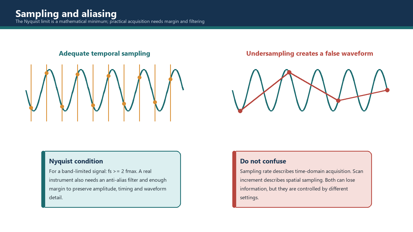
Aliasing: False frequency content created when the sampled signal contains frequencies that cannot be represented by the selected sampling system.
Anti-alias filter: An analogue filter before the ADC that limits frequency content entering the sampler.
Point quantity: The number of stored sample points in an A-scan or selected acquisition range.
Raw payload estimate: A calculation of basic sample bits before file headers, metadata, packing, derived data, compression and other implementation details.
4.1 From voltage to numbers
The returning ultrasonic signal at a receiver channel is initially an analogue voltage that varies with time. A digital system cannot store a continuous voltage. It measures the voltage at discrete instants and assigns a numerical value to each measurement.
Two independent choices affect that representation:
- Sampling frequency controls how closely the measurements are spaced in time.
- Bit depth controls how many numerical levels are available for each measurement.
More samples can describe faster waveform changes. More bit depth can describe smaller amplitude steps within the converter's input range. Neither automatically improves the physical sound beam, coupling or reflector response. They affect the numerical representation of the received signal.
4.2 Bit depth and quantisation levels
For an ideal b-bit converter, the number of available codes is:
Number of codes = 2^b
| Bit depth | Available codes |
|---|---|
| 8 bit | 256 |
| 10 bit | 1,024 |
| 12 bit | 4,096 |
| 16 bit | 65,536 |
These totals do not, by themselves, state how values are stored or displayed. An instrument may map the codes to an unsigned range, a signed radio-frequency range, a rectified amplitude range or an internally scaled value. A 12-bit ADC therefore means 4,096 possible converter codes; it does not guarantee that the file packs every sample into exactly 12 physical bits or that the display exposes all 4,096 levels.
Quantisation introduces a small difference between the original analogue voltage and its assigned code. Increasing bit depth reduces the ideal code step for the same full input range, but practical accuracy also depends on electrical noise, converter performance, analogue gain, clipping and subsequent processing.
Worked example 4.1 - comparing bit depths
A 10-bit converter provides 2^10 = 1,024 codes. A 12-bit converter provides 2^12 = 4,096 codes.
The 12-bit converter offers four times as many ideal amplitude codes because 4,096 / 1,024 = 4. It does not provide four times the ultrasonic resolution. Axial and lateral resolution depend on pulse and beam characteristics, while the useful amplitude precision depends on the full signal chain.
4.3 Sampling a waveform in time
For a sinusoidal component of frequency f:
Cycle period, T = 1 / f
If n samples are taken during each temporal cycle:
Sample interval, T_s = T / n
Sampling frequency, f_s = 1 / T_s = n f
The phrase temporal cycle is deliberate. It describes samples across the waveform period at a fixed channel. It is not the same as spatial scan increment along the component, and it is not the number of elements in one wavelength across an array.
Worked example 4.2 - a course sampling convention
Assume a 4 MHz sinusoidal component and a selected convention of five samples per temporal cycle.
- Cycle period: T = 1 / 4 MHz = 0.25 microseconds.
- Sample interval: T_s = 0.25 / 5 = 0.05 microseconds.
- Sampling frequency: f_s = 1 / 0.05 microseconds = 20 MHz.
The same result follows directly from f_s = n f = 5 x 4 MHz = 20 MHz.
Five samples per nominal probe-frequency cycle is a training or procedure convention, not the Nyquist theorem and not a universal equipment requirement. The required sampling design must consider the highest relevant frequency in the received bandwidth, the anti-alias filter, the instrument architecture and the governing procedure.
4.4 Nyquist rate, Nyquist frequency and aliasing
For an ideal band-limited signal, a necessary lower boundary for sampling is:
f_s >= 2 f_max
where:
- f_s is the sampling frequency;
- f_max is the highest signal frequency that must be represented.
The Nyquist rate for that signal is 2 f_max. The Nyquist frequency of a sampling system is:
f_N = f_s / 2
The terms answer different questions:
- Nyquist rate asks, "What ideal minimum sample rate corresponds to this highest signal frequency?"
- Nyquist frequency asks, "What is the highest ideal frequency boundary for this selected sample rate?"
Why twice is not a comfortable practical target
The equality f_s = 2 f_max is an ideal mathematical boundary. At exactly two samples per cycle, sample phase can produce a poor description of amplitude and waveform shape. Real signals contain a band of frequencies, real filters have transition bands, and practical systems require margin.
An anti-alias filter limits the frequency content before sampling. The selected f_s must be high enough that the frequencies allowed through that filter and needed for the inspection fall within the usable sampled bandwidth. The practical choice may be significantly higher than twice the nominal probe frequency.
Continue Example 4.2. At f_s = 20 MHz, the Nyquist frequency is 10 MHz. If the highest relevant received component after analogue filtering is 7 MHz, the ideal Nyquist rate is 14 MHz and the 20 MHz selection is above that lower boundary. If relevant 12 MHz content enters the ADC, a 20 MHz sampling frequency is insufficient because 12 MHz is above the 10 MHz Nyquist frequency.
Aliasing is not repaired by smoothing the displayed waveform. Once out-of-band energy has been sampled into a false in-band pattern, later processing cannot reliably reconstruct what the ADC failed to represent.
4.5 Analogue and digital filtering
Filters select or reduce frequency regions. Their location and purpose should be identified.
Analogue anti-alias filtering
This filter acts before digitisation. Its task is to attenuate frequency content that the selected ADC sampling system cannot represent reliably. It is part of the acquisition design.
High-pass filtering
A high-pass filter reduces lower-frequency components while passing frequencies above its transition region. It may reduce low-frequency drift or unwanted low-frequency response, but it can also alter a legitimate broadband echo.
Low-pass filtering
A low-pass filter reduces higher-frequency components. It may reduce high-frequency noise, but excessive filtering can remove useful high-frequency content and lengthen or reshape the apparent pulse.
Band-pass filtering
A band-pass filter retains a selected frequency band and attenuates frequencies below and above it. The band should suit the useful probe response and inspection objective.
Band-stop or notch filtering
A band-stop filter suppresses a selected frequency region. It may be useful for a known interference source, but it can also remove part of the ultrasonic response.
Filtering can improve the visible signal-to-noise ratio, yet any change can affect amplitude, waveform shape and sensitivity. Required filters should be selected before sensitivity calibration. If a filter is changed after calibration, the setup must be re-evaluated and recalibrated as required.
4.6 Rectification, smoothing and display processing
An RF A-scan contains positive and negative voltage excursions. Rectification may show the positive portion, negative portion or a full-wave magnitude representation. An envelope or smoothing function may then create a slower contour around the rectified response.
These functions can make a display easier to read, but they can also change the apparent peak, pulse width and separation between nearby responses. Two close peaks may merge. A small high-frequency response may be reduced. It is unsafe to promise that a crack response will always survive smoothing simply because it is a real reflector.
Smoothing does not reduce the ADC sampling frequency required to prevent aliasing. It also does not inherently reduce a stored raw file. Either effect would depend on the instrument's acquisition and storage implementation. The operator must establish what the system acquires, what it stores and which display operations are reversible.
4.7 Acquired, stored, processed and displayed data
The word raw is used loosely in industry. It may mean individual element-channel samples, a beamformed RF A-scan before rectification, a stored A-scan before display processing, or simply the least processed file available from a particular instrument.
For a controlled inspection, define the data stages:
- Acquired channel data: Samples created by the ADCs before or during beamforming, if available.
- Beamformed A-scan: The delayed and summed response for one focal law.
- Stored inspection data: The waveforms, gated values, positions, setup and metadata actually written to the file.
- Processed data: Results after rectification, filtering, smoothing, compression, averaging or geometric correction.
- Displayed data: A view rendered with selected colour map, gain, range, gates, cursors and screen resolution.
The stored file may not contain every earlier stage. If only gated peak values are stored, the complete waveform cannot later be recovered. If full A-scans are stored, offline display settings may be adjustable, but acquisition-stage filtering may still be irreversible.
Documenting this boundary is essential when data is reviewed by another technician or used as permanent inspection evidence.
4.8 What drives file size
A raw-payload estimate grows with the following main factors:
- bit depth or stored word size;
- point quantity per A-scan;
- number of focal laws;
- number of groups or probes;
- number of encoded acquisition positions;
- scan length;
- finer scan increment, because it increases position count;
- full-waveform storage rather than selected gated values.
Processing and compression may change final file size, but their effect is implementation-dependent. Smoothing must not be used as a generic file-size control claim.
For one group with a constant point quantity and law count:
Raw payload bits = b x P x N_laws x N_positions
where:
- b = stored bits per sample in the estimate;
- P = points per stored A-scan;
- N_laws = stored laws per position;
- N_positions = integer encoded positions.
For multiple groups with different configurations, calculate each group's payload and sum the results. If the file stores a 12-bit converter value in a 16-bit word, use 16 stored bits for a realistic payload estimate or clearly label the 12-bit result as a lower-level converter estimate.
4.9 Counting integer acquisition positions
A data position cannot be fractional. The count depends on the endpoint convention.
If a scan begins at 0 mm, ends at L, stores both endpoints, and L is exactly divisible by increment Delta x:
N_positions = L / Delta x + 1
The number of increments is L / Delta x; the number of positions is one greater because the start is also stored.
If L is not exactly divisible by Delta x, state how the system handles the endpoint:
- storing positions from zero without exceeding L gives floor(L / Delta x) + 1 positions;
- guaranteeing a final point at L without exceeding the maximum spacing may require ceiling(L / Delta x) + 1 positions and an adjusted final interval;
- some encoder systems stop at the last triggered increment and do not force a sample at the exact nominal end.
The convention must be declared before calculating file size or claiming coverage.
4.10 Binary and decimal storage units
Use unit names consistently:
- 8 bits = 1 byte;
- 1 KiB = 1,024 bytes;
- 1 MiB = 1,024 KiB = 1,048,576 bytes;
- 1 kB = 1,000 bytes;
- 1 MB = 1,000,000 bytes.
Lowercase b denotes bits; uppercase B denotes bytes. A value written only as "36 mb" is ambiguous twice: it confuses bit/byte case and does not state decimal or binary scaling.
For binary conversion:
KiB = bits / (8 x 1,024)
MiB = bits / (8 x 1,024 x 1,024)
For decimal conversion:
MB = bits / (8 x 1,000,000)
4.11 Worked file-size example
A group uses:
- 12-bit converter values in the lower-level estimate;
- 512 stored points per A-scan;
- 40 laws;
- a 240 mm encoded scan;
- 0.5 mm spacing;
- both 0 mm and 240 mm positions stored.
Because 240 / 0.5 = 480 increments:
N_positions = 480 + 1 = 481.
Raw bits = 12 x 512 x 40 x 481 = 118,210,560 bits.
Raw bytes = 118,210,560 / 8 = 14,776,320 bytes.
Binary size = 14,776,320 / 1,024 = 14,430 KiB = approximately 14.09 MiB.
Decimal size = 14,776,320 / 1,000,000 = approximately 14.78 MB.
This is not a prediction of the final vendor file. Headers, setup data, encoder records, gates, measurements, derived images, sample packing, extra groups and compression can all change the result. The estimate is useful for comparing setup choices and checking whether a planned scan is plausible.
4.12 Planning data rather than discovering limits mid-scan
Before acquisition, the Level 2 technician should confirm:
- the instrument's actual file and storage limits for the installed software/firmware;
- point quantity and range required to capture the inspection volume;
- total laws and groups;
- encoded length and integer position count;
- sample packing and waveform-storage mode where known;
- expected file count if the inspection must be divided;
- transfer, backup, naming and retention arrangements;
- whether the analysis workstation can handle the resulting data efficiently.
Reducing data should be a controlled decision. A coarser increment, fewer laws, shorter range or gated-only storage may reduce file size, but each can also reduce coverage, angular information, waveform evidence or location detail. Storage convenience must not silently rewrite the inspection objective.
Common traps
- Calling bit depth ultrasonic resolution. It describes numerical amplitude levels, not physical reflector separation.
- Using nominal probe frequency as f_max without considering bandwidth. Anti-alias design depends on the highest relevant received frequency.
- Calling 2 f_max a comfortable practical sample rate. It is the ideal Nyquist lower boundary.
- Confusing Nyquist rate with Nyquist frequency. One is 2 f_max; the other is f_s / 2.
- Expecting digital smoothing to prevent aliasing. Aliasing must be controlled before or at sampling.
- Assuming displayed data equals stored data. Display processing and file contents may differ.
- Using a fractional number of scan positions. Declare the endpoint rule and use an integer count.
- Mixing MB, MiB, bits and bytes. State the unit system and use letter case correctly.
- Ignoring packing and metadata. The raw payload formula is an estimate, not a file guarantee.
Chapter summary
An ADC samples an analogue waveform in time and maps each sample to one of 2^b codes. Sampling frequency controls temporal spacing; bit depth controls the ideal number of amplitude codes. For a sinusoidal component, T = 1/f, T_s = T/n and f_s = n f.
The ideal Nyquist condition is f_s >= 2 f_max. Nyquist rate is 2 f_max, while Nyquist frequency is f_s/2. Practical sampling also requires an analogue anti-alias filter and margin for bandwidth and filter transition.
Filtering, rectification and smoothing can improve presentation but can also change amplitude and waveform detail. The technician must know what is acquired, stored, processed and displayed. Raw file-size estimates require bit depth, A-scan point quantity, law count and an integer position count. Binary KiB/MiB and decimal kB/MB must not be mixed.
Study and revision only. This is not an approved inspection procedure, acceptance criterion or qualification.