
CHAPTER 6 · Ultrasonics Level 1
Reading Your First A-Scan Properly
In this chapter · 18 sections
Why this matters
An A-scan can contain an initial disturbance, several echoes and a moving baseline. It is tempting to treat every peak as an object drawn inside the component. That is not what the display shows. It shows processed receiver response against time or a calculated distance. Correct reading begins with the axes, then checks timing, repeatability, movement, back-wall behaviour and system state. This chapter turns the A-scan from a collection of spikes into a traceable piece of evidence.
What you already need
- A pulse travels out and an echo can return.
- The probe and instrument form one signal chain.
- Sound speed and round-trip time support a distance estimate.
- Gain changes displayed response, not reflector size.
What you will learn
- Identify the main landmarks on a straight-beam A-scan.
- Separate range, velocity, zero and display delay.
- Explain gain, radio-frequency (RF), rectified and envelope displays.
- Recognise dead zone, noise, saturation, multiples and wrap-around.
- Use echo patterns and probe movement to test echo identity.
- Describe an A-scan observation without overclaiming its cause.
Words you will meet
- Range: time or distance span represented on the display.
- Zero: correction for time before the intended component path begins.
- Gate: selected time region used for measurement or alarms.
- Dead zone: early region where recovery or ringing hides useful echoes.
- Saturation: overload that clips or distorts the true signal.
6.1 Axes and the main landmarks
An A-scan is a graph. The horizontal axis begins as time. The vertical axis shows a signal-derived amplitude. An instrument can relabel time as sound path, depth or thickness only after it applies a selected velocity, starting correction and path model.
The earliest part often contains a large initial pulse or interface response. A region immediately after it can be difficult to inspect because the probe and receiver are still recovering. A response from the far surface appears later and is called the back-wall echo. In a parallel low-loss component, sound can bounce again and create second and third back-wall echoes.
The following figure labels a simple trace. Notice that the gate is a measurement window placed over part of the A-scan. It is not a box drawn around a physical flaw.
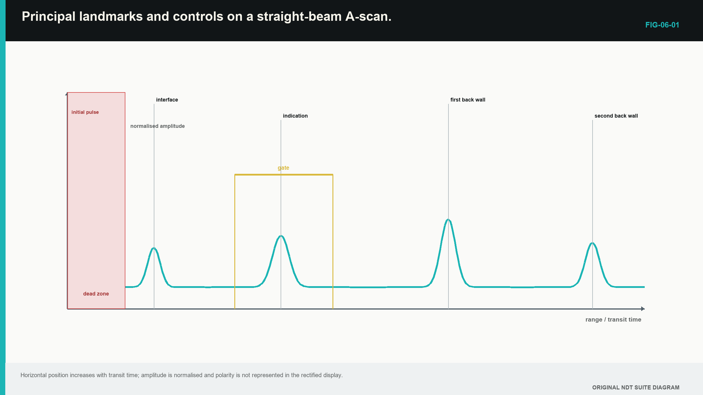
Horizontal position helps answer “when did this response arrive?” A path and velocity model are then needed to estimate where it occurred. Vertical height answers “how large was the received electrical response under this setup?” It does not directly give reflector dimensions.
Multiple back-wall echoes provide useful pattern evidence. Their spacing should be approximately equal because each new echo adds another round trip through the same wall. Unequal spacing can point to a wrong peak, a different boundary, layering, changing thickness, mode conversion or a poor timing model.
A sensible first reading uses a fixed order. Start at the left and identify the transmitted or interface region. Move right and locate the first plausible component echo, then look for a matching repeat interval.
Check whether the horizontal scale says time, sound path or thickness. Check whether the vertical scale is raw RF, rectified response or an envelope. Finally, move the probe slightly and watch which features remain stable. This routine slows the learner down by a few seconds and prevents a surprisingly large collection of confident mistakes.
Begin with a simple parallel block when possible. Couple the probe, find the first back-wall echo and reduce the range until that echo and at least one repeat are easy to see. Do not chase a perfect height yet. First confirm that both peaks move together when display delay changes and keep the same spacing when gain changes.
Now lift and replace the probe. The times should return closely if the same wall is being measured. Heights may vary because the couplant film changed. This separates a timing landmark from an amplitude condition. The learner can then introduce a gate around the intended echo and confirm that the gate number follows that visible peak.
This small exercise connects the physical plate to the screen. The left-to-right trace is no longer a row of unexplained spikes. It becomes a transmit region, one wall round trip and a second round trip. That concrete pattern should be secure before unusual echoes or automatic measurements are interpreted.
6.2 Range, velocity, zero and display delay
Four controls that can move or reframe echoes must be kept separate.
Range controls how much time or calculated distance the screen shows. Increasing range lets later echoes appear but compresses the same information into the display width.
Velocity controls the time-to-distance scale. If selected velocity is 2% too high, calculated distances are about 2% too high in a simple linear model. The error grows with distance.
Zero or probe-delay correction removes time spent before the intended component path. That time can occur in the probe wear face, a delay line, a wedge or electronics. A zero error creates an approximately constant distance offset.
Display delay shifts the visible window along the existing time record when used correctly. It should not silently change the physical zero model.
The simple pulse-echo distance model can include a fixed time offset. In words:
displayed distance = assumed speed × corrected round-trip time ÷ 2
| (6.1) Linear distance model with zero offset · EQ-06-01 Where: d_display = displayed pulse-echo distance (m); c_assumed = selected speed (m/s); t_measured = measured transit time (s); t_zero = system delay represented as time (s) Model limits: one effective speed and a pulse-echo path; correctly identified echo |
|---|
One known reflector can be made to appear in the right place by several combinations of speed and zero. Two known paths provide more information. A zero problem shifts both by a similar amount. A scale problem produces a larger error at the longer path.
| Worked example · Separating zero error from scale error WE-06-01 Given: A reference piece has reflectors at true paths of 25.0 mm and 75.0 mm. The instrument reads 27.0 mm and 79.0 mm. Find: Whether a constant zero shift alone explains the readings. Steps: Find each error. At 25.0 mm: 27.0 - 25.0 = +2.0 mm. At 75.0 mm: 79.0 - 75.0 = +4.0 mm. Answer: The error is not constant. A zero shift alone cannot explain it. A scale or velocity error is present, possibly together with a zero error. What this tells you: Two known points reveal a distorted scale that one point could hide. Common mistake: Adjusting zero at the first reflector and assuming the complete distance scale must then be correct. |
|---|
6.3 Gain, waveform views and gates
Gain amplifies receiver voltage. More gain can make a weak response visible. It also raises noise. If the receiver or digitiser overloads, the waveform can flatten and useful amplitude information is lost.
A radio-frequency (RF) display shows positive and negative oscillations. It preserves polarity and cycle detail. Full-wave rectification turns both signs upward. An envelope view smooths the carrier oscillations into an outline. Rectified and envelope views are easier to read for many routine tasks, but they remove phase or cycle information.
The selected view can change the reported time. An RF peak, envelope peak and threshold crossing need not occur at the same instant. Filters and smoothing can shift or broaden the response. When two readings are compared, their processing must also be comparable.
A gate selects a time window. The instrument may measure the highest peak, first threshold crossing or another feature inside it. Gate start, width and threshold should include the intended echo and exclude unrelated signals where practical.
The gate does not know which reflector produced a peak. If a stronger geometry echo enters the window, a peak-tracking measurement can jump to it. If noise crosses the threshold first, a first-crossing measurement can report noise. The retained A-scan is needed to check what the number followed.
6.4 Dead zone, noise and false responses
The probe continues ringing for a short time after excitation. The receiver also needs time to recover from the large transmit event. Together, these can hide early component echoes. The obscured region is called dead zone.
A delay line or dual-element probe can move the useful component interval away from the initial disturbance. That solution brings its own delay or V-path geometry, so it must be calibrated over the intended range.
Noise has different causes. Random electronics can create a restless baseline. Electromagnetic pickup can repeat with equipment activity. Material grains can return real acoustic energy called structural noise. Poor coupling can make the whole trace rise and fall. These causes should not all be treated as one “noisy screen” problem.
Other responses can arrive at unexpected times:
- wedge or delay-line echoes;
- repeated interface echoes;
- mode-converted paths;
- repeated back-wall paths;
- geometry reflections;
- echoes from an earlier pulse when pulse repetition is too fast.
The last effect is commonly called wrap-around. A long-path echo from one firing can arrive after the next firing begins, so the instrument places it at a false position in the new time window. Changing pulse repetition frequency, or PRF, changes that apparent position.
6.5 Echo identity from patterns and movement
Time tells us where an echo could fit under one model. It rarely proves identity by itself. Useful supporting evidence includes repeatability, back-wall behaviour, probe movement, known geometry and response from another direction.
A true back-wall echo in uniform parallel plate usually remains at about the same depth as the probe moves. Its amplitude can change with coupling or surface condition. A side-drilled hole response rises and falls as the beam crosses it. A component edge can trace a predictable curve. Fine structural-noise peaks often change over small movement.
Several adjacent A-scans reveal continuity. A B-scan can present the same information as a section, but it is still assembled from individual time signals. Interpolation can make widely spaced samples look smooth, so the underlying spacing remains important.
Echo trains add another identity clue. Equal spacing supports repeated travel between the same boundaries. An internal flat reflector can produce its own series. If responses appear at 30, 60 and 90 mm while the expected back wall is 50 mm, an internal boundary is more plausible than three unrelated flaws.
| Worked example · Using multiple-echo spacing WE-06-02 Given: Peaks occur at 16.9, 33.8 and 50.7 microseconds after an unknown fixed probe delay. Use 5,900 m/s. Find: Thickness from the spacing between echoes. Steps: Each adjacent spacing is 16.9 microseconds. That spacing represents one extra round trip through the wall. d = (5,900 m/s)(16.9 x 10^-6 s)/2 d = 0.0499 m = 49.9 mm Answer: Estimated thickness is 49.9 mm. What this tells you: The unknown fixed probe delay cancels because the calculation uses the interval between successive echoes. Common mistake: Using the method without checking that all peaks come from the same pair of boundaries. |
|---|
6.6 Step up preview - automatic measurement is a rule
A gate can report a peak or another selected point, and that selected point can change when nearby echoes or signal height change. Level 1 therefore checks the visible waveform before accepting an automatic number. The detailed peak, threshold, correlation, noise-window and timing-bias treatment moves to Level 2.
Digital instruments also record the waveform as samples. The sample rate and filtering must suit the signal to avoid false frequency content, as developed by the cited sampling source. [R005] The Level 1 requirement is practical: use the equipment within its supported setup and retain enough waveform information to review the reading; no sampling-theorem calculation is assessed here.
6.7 Recognising error signatures
Different faults leave different patterns. The figure compares five common signatures. Notice that some move echo time, some change amplitude and some destroy shape.
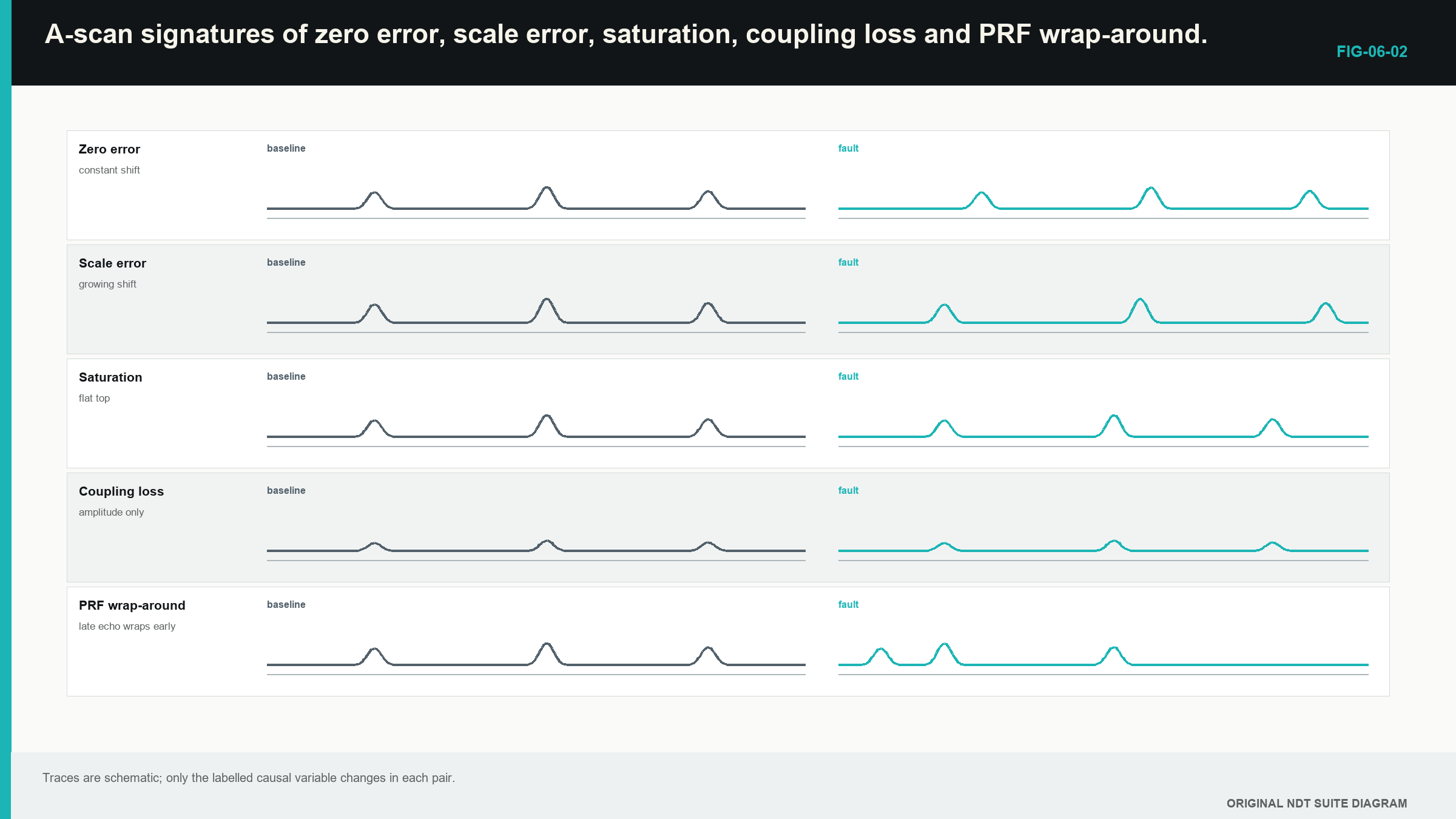
- If all echo times shift by a similar amount, zero or trigger delay is plausible.
- If distance error grows with range, velocity or time-base scale is plausible.
- If all echo heights fall together, coupling or common sensitivity is plausible.
- If large peaks become flat and stop rising with gain, saturation is plausible.
- If a late echo changes apparent time when PRF changes, wrap-around is plausible.
- If the trace changes when the cable moves, connector or shielding trouble is plausible.
Saturation can occur before the display. If the analogue receiver clips, reducing display scale later does not recover the lost waveform. A flat top, added frequency components or an unchanging peak as gain rises can reveal clipping. A 6 dB drop measured from a clipped maximum is not a true half-amplitude point.
A large early signal can also disturb receiver recovery and suppress later weak echoes. A late echo disappearing after a strong front-surface event may be receiver behaviour rather than material absorption.
Good diagnosis changes one control at a time and predicts the result. Changing range, gain, delay and PRF together may remove the troubling echo, but it also removes the evidence that identified the cause. Tiny gremlins thrive in undocumented knob-twiddling.
6.8 Describing and preserving the evidence
A useful A-scan description states acquisition condition, timing model and observations. For example:
A repeatable unsaturated response appears 12 microseconds after the interface. It peaks at the stated probe coordinate and is accompanied by a reduced back-wall echo.
That statement gives another reader something to test. A following interpretation can list causes consistent with the response, such as an internal boundary, geometry or a mode-converted path. It should also state the next evidence that separates them.
A screenshot alone often omits sample rate, filter, gain, zero, gate logic and RF polarity. A stored waveform with its settings supports later remeasurement. Automated systems should retain enough waveform evidence to explain why a numeric result changed.
Consider a late response that repeats over three nearby probe positions. Its time is stable and the back wall is stable. Increasing PRF moves it earlier. Spatial repeatability might first suggest a component feature, while PRF dependence suggests wrap-around. The contradiction is valuable. The next test keeps acquisition identity and changes PRF in a controlled way. Only after the timing mechanism is resolved should geometry be used to name the reflector.
An A-scan is therefore both a measurement display and a diagnostic record. Its strongest reading combines time, pattern, movement, geometry, processing state and a clear boundary between observation and conclusion.
The A-scan and pulse-echo foundation in this chapter follows the cited international and foundational sources. [R001] [R002]
In plain words
- An A-scan plots received response against time or a calculated distance.
- Range, velocity, zero and display delay perform different jobs.
- Gain makes voltage larger but does not improve pulse or beam resolution.
- RF, rectified and envelope displays retain different signal details.
- A gate selects a time region; it does not identify the reflector.
- Echo trains and probe movement provide stronger identity evidence than one peak.
- Saturation, noise, dead zone and wrap-around can create convincing false readings.
- A saved waveform and its settings are more useful than an unexplained screenshot.
Key terms
- Range: span shown along the time or distance axis.
- Zero: correction for time before the intended component path.
- Gate: time window used for measurement or alarms.
- Dead zone: early interval hidden by ringing or recovery.
- Saturation: overload that distorts the signal.
- PRF: number of pulse-and-receive cycles started each second.
Key relationships
- d_display = c_assumed(t_measured-t_zero)/2: displayed pulse-echo distance uses corrected round-trip time and an assumed speed.
- Equal back-wall echo spacing can support a repeated path through the same wall.
- A constant distance error suggests zero; an error that grows with range suggests scale or velocity.
Common mix-ups
- The horizontal axis is not automatically physical depth.
- Display delay is not the same as probe-zero correction.
- A gate value is not proof of correct echo identity.
- A smooth trace is not proof of unlimited sampling resolution.
- Lowering display height after analogue saturation does not restore the waveform.
Bridge to Chapter 7
This chapter taught how to identify and challenge A-scan responses. Chapter 7 applies that skill to straight-beam thickness and lamination work. The arithmetic remains simple; the harder task is deciding which echo represents the real wall and how completely the area was sampled.
Sources and further study
- [R001]
- [R002]
- [R005]
CLASSROOM LAB · INTERACTIVE
Try the A-scan
Move the reflector and compare the physical depth with echo time. This is a simplified teaching model, not a calibration or inspection calculation.
Open the full classroom lab ↗Study and revision only. This is not an approved inspection procedure, acceptance criterion or qualification.