
CHAPTER 23 · Ultrasonics Level 3
From Demonstration Results to Reliability and POD
In this chapter · 23 sections
Why this matters
A technique detects 19 of 20 known targets; the observed detection fraction is 95%, but that number is not yet proof of 95% probability of detection across production components. The trials may be few, clustered in one specimen, completed by one operator or concentrated at easy target sizes. Level 3 must separate the count that was observed, the population behaviour being estimated and the uncertainty in that estimate. This chapter builds that staircase slowly, then connects it to false calls, sizing reliability, qualification and model-assisted evidence.
What you already need
- The bounded technique claim and target population from Chapter 22.
- The difference between repeatability and reproducibility.
- Fractions, percentages, graphs and simple algebra.
- Familiarity with detection thresholds and false indications.
- The idea that sample evidence may not represent every production condition.
What you will learn
- Distinguish detection count, observed fraction, probability and confidence.
- Explain hit-miss and signal-response study designs.
- Read a POD curve and a lower confidence bound without overclaiming.
- Include false calls, operator variation and clustering in reliability reasoning.
- Separate feasibility, qualification, routine verification and sizing reliability.
- State the evidence boundary of physical and model-assisted POD programmes.
Words you will meet
- Detection fraction: number detected divided by number eligible in the observed trials.
- Probability of detection: population model for detection under stated conditions.
- Confidence bound: conservative statistical boundary reflecting finite study data.
- Hit-miss data: binary detected or not-detected outcome for each eligible target.
- Signal-response data: retained continuous response used with a declared decision threshold.
- False call: detection decision associated with an unflawed decision region.
- Clustering: dependence created when trials share flaw, specimen, operator or setup.
- Random effect: modelled variation among sampled groups such as operators or specimens.
- POD: abbreviation for probability of detection.
- MAPOD: model-assisted probability of detection.
Depth guide for this chapter
- Understand here: the meaning, assumptions and limits of reliability evidence.
- Calculate here: observed fractions, simple confidence intervals, bias and threshold trade-offs.
- Derive later: logistic fitting, formal probability fitting, random effects, probability updating and formal MAPOD integration are developed in Chapters 64 and 78.
23.1 Begin with twenty visible outcomes
Imagine twenty cards placed in flaw-size order; nineteen are marked detected and one is marked missed. The first fact is the count. Nineteen eligible trials produced a detection, and one did not. The observed detection fraction is calculated as follows.
| (23.1) Observed hit fraction · EQ-23-02 Where: p_hat = observed fraction; k = detected trials; n = eligible trials Model limits: descriptive statistic only; does not by itself establish population POD or confidence |
|---|
For this set, p_hat = 19/20 = 0.95; that is a correct description of the data. It does not state the true detection probability for all relevant flaws, components and operators. A different sample of twenty can produce a different fraction even when drawn from the same stable population. The arrangement of the cards matters; if the missed target is among the smallest and the larger targets are all detected, size dependence is plausible. If all twenty presentations are repeated scans of one notch, the data mostly describe repeatability. If twenty different natural flaws across several components and operators were used, the data contain broader population information. Equal counts can support unequal claims.
NASA guidance emphasises that POD belongs to a defined inspection system and population, including specimens, flaws, operators and analysis. [R034] It is not a permanent label attached to ultrasonic testing, a probe model or a procedure title.
23.2 Observed fraction, probability and confidence
Three terms must remain separate. The detection fraction is observed data. Probability of detection, or POD, is a model for future or population outcomes under stated conditions; a confidence bound reflects uncertainty in the fitted population model because the study is finite.
Even under the simplest case of independent identical trials, 19 successes do not establish an exact 0.95 population probability; a confidence interval shows how wide the supported range remains. A Bernoulli trial has two possible outcomes, such as detected or missed. A Wilson interval is one method for estimating a probability range from a finite binary count.
| Worked example · Why nineteen out of twenty is not a 95 percent guarantee WE-23-01 Given: Nineteen successes in twenty independent, identical Bernoulli trials. Use the 95% Wilson interval with p_hat = 0.95, n = 20 and z = 1.96. Find: The approximate interval for the underlying probability under this simplified model. Steps: Wilson centre numerator is p_hat + z^2/(2n) = 1.0460. Denominator is 1 + z^2/n = 1.1921. Half-width numerator is z sqrt(p_hat(1-p_hat)/n + z^2/(4n^2)) = 0.1355. Divide centre and half-width by the denominator. Answer: Approximate 95% interval is (1.0460 +/- 0.1355)/1.1921, or about 0.764 to 0.991. Technical implication: Twenty trials leave substantial uncertainty even before flaw size, representativeness and clustering are considered. Common mistake: Reporting the point estimate as a guaranteed population performance ignores finite-sample uncertainty. |
|---|
The calculation is included so the learner can interpret a supplied confidence result; deriving Wilson intervals, selecting among interval methods and handling clustered trials belong to Chapter 64.9 and Chapter 78.
23.3 Hit-miss and signal-response evidence
A hit-miss study assigns each known target a binary outcome under a declared call rule; the method is direct and accommodates outcomes that cannot be represented by one amplitude. It discards how far above or below threshold a response fell. A signal-response study retains a continuous metric related to target size, such as amplitude or another declared feature; a threshold converts the metric into a detection decision. This approach can retain more information, but it assumes the response model, noise behaviour and threshold remain meaningful.
Both designs need credible truth; artificial targets give known geometry and repeatability but may not represent natural crack morphology. Natural flaws provide realistic acoustic interaction while adding truth uncertainty. A mixed programme can use each for its strongest role when differences remain explicit. Size is usually only one explanatory variable; orientation, depth, roughness, material noise, surface, equipment and operator can shift response at the same size. A one-dimensional POD curve averages over the factor distribution in the study. It transfers only when the production distribution is compatible or the influential factors are represented separately.
23.4 Build a POD curve gradually
For a hit-miss study, plot each result against the declared flaw-size measure; a row of misses at small sizes, mixed outcomes in a transition region and mostly hits at larger sizes suggests a rising probability. A fitted curve summarises that trend. A common formal model is logistic regression.
| (23.2) Logistic hit-miss POD model · EQ-23-01 Where: POD(a) = probability of detection at flaw size a; beta_0 and beta_1 = fitted coefficients; a = declared flaw-size measure Model limits: independent Bernoulli outcomes conditional on size, suitable logistic relationship and representative study population |
|---|
At Level 3, the learner should interpret the curve and its assumptions. beta_0 shifts the transition, while beta_1 controls how sharply the probability rises with size. The model does not prove that size is the only influence or that detection must follow this exact shape. The figure below shows individual observations, a fitted curve and a lower confidence bound; notice that the tested size range is marked. Behaviour beyond that range is extrapolation.
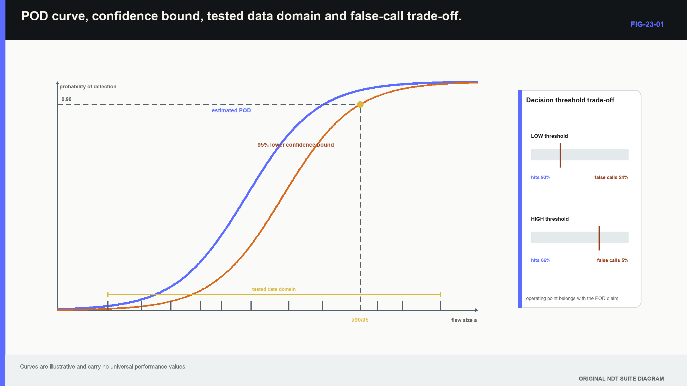
The term a90/95 commonly describes the flaw size where the lower 95% confidence bound reaches 90% POD under the chosen study and model; it is not a universal crack size detected 90% of the time. It remains conditional on flaw measure, population, system, analysis and statistical method. Complete separation can occur when every small flaw is missed and every large flaw is detected; the pattern looks ideal, but ordinary logistic coefficients can become unstable because little information exists inside the transition. Additional targets near that transition can be more informative than many obvious misses and obvious hits.
Plots should show individual observations, not only a fitted line; grouping by operator, specimen and material can expose hidden patterns. A smooth curve can otherwise conceal that one operator or one component produced most misses.
23.5 Thresholds and false calls
A detection threshold divides a continuous evidence space; lowering it usually increases both true detections and false calls. The technically suitable operating point depends on consequences, follow-up resources and governing requirements, not on a curve alone. False-call rate needs a denominator; it can be reported per component, scan length, unflawed region or defined decision opportunity. Each answers a different planning question. Counting only implanted-flaw positions ignores geometry calls elsewhere. Treating every neighbouring image pixel as independent exaggerates the denominator because image samples are correlated.
Receiver-operating-characteristic analysis compares true-positive and false-positive behaviour across thresholds; it does not choose the engineering threshold. Precision-recall views can help when flaws are rare, but they also depend on labelled truth and the population mix.
| Worked example · Comparing two thresholds with explicit false calls WE-23-03 Given: A trial includes 40 flaws and 200 defined unflawed decision regions. Threshold A calls 36 flaws and produces 30 false calls. Threshold B calls 32 flaws and produces 8 false calls. Find: Observed sensitivity and false-positive proportion at each threshold. Steps: For A, sensitivity is 36/40 = 0.90, and false-positive proportion is 30/200 = 0.15. For B, sensitivity is 32/40 = 0.80, and false-positive proportion is 8/200 = 0.04. Answer: Threshold A gains 10 percentage points of observed sensitivity and adds 11 percentage points of false-positive proportion relative to B. Technical implication: The trial exposes a trade-off. Confidence, flaw-size distribution and decision consequence are still required to select an operating threshold. Common mistake: Selecting the threshold on the same development data and reporting that performance without independent evaluation creates optimistic evidence. |
|---|
Production prevalence can differ greatly from a flaw-rich trial; when most regions are unflawed, even a modest false-call proportion can dominate follow-up work. Threshold development should therefore include realistic geometry and unflawed regions, not only implanted targets.
23.6 Study design and independence
Representative variation should include factors expected in use; flaw sizes, orientations and morphologies; material batches; surfaces; geometry; operators; equipment; and environment can all matter. A fully crossed design may be impractical, so stratification, blocking and randomisation distribute the important variation. Blind presentation reduces expectation bias; training and practice cases should remain separate from scored trials. Random order reduces the chance that learning or fatigue follows flaw size. The actual information available to a production analyst should be reproduced when human performance is part of the claim.
Clustering occurs when observations share a flaw, specimen, operator or setup; ten scans of one flaw by one operator do not equal ten independent flaws. Those repeats can estimate within-flaw or within-operator variation. They cannot be treated as independent population trials without a model that represents the shared source. A random effect represents variation among sampled groups such as operators or specimens; with enough groups and observations, a model can separate average performance and between-group spread. With two operators, broad claims about the operator population remain weak regardless of how many times each scans the same flaws.
Human and automation performance should be evaluated as the combined decision system intended for use; an algorithm that proposes candidates and a person who confirms them do not have a POD obtained by simply adding their separate values. Information flow, automation bias, threshold and review rules shape the combined result.
23.7 Plan information near the transition
A POD study gains much of its information where outcomes change from mostly missed to mostly detected; a study containing only easy large flaws cannot locate the lower capability boundary. A study containing only very small misses cannot describe upper behaviour. Preliminary trials or physical models can help choose sizes that span the transition and remain relevant to the engineering need. Sample planning depends on required confidence, expected slope, clustering and available variation; there is no universal count that makes every study adequate. More independent flaws often add population information, while repeat presentations help quantify operator or setup contributions. Allocation follows the uncertainty that matters to the claim.
Public reliability frameworks describe POD and model-assisted study principles. [R033] [R034] Method-specific work also illustrates the need to define response, noise and population. [R052] These resources support disciplined design; merely naming the framework does not make an unrepresentative dataset representative.
23.8 Feasibility, qualification and routine checks
A feasibility demonstration establishes that a concept can produce useful evidence; a qualification programme supports stated performance across a defined domain. Routine verification establishes that selected features of the deployed system remain consistent with the qualified state. These activities differ in scale because they answer different questions; a reference-block echo can support system condition. It is not a POD study. Repeating a full population study every shift is unnecessary when sensitive routine indicators are controlled. A major change to coverage, threshold or interpretation may require targeted bridging or renewed reliability evidence.
MIL-HDBK-1823A supplies a recognised reliability-assessment framework that includes ultrasonic and model-assisted contexts. [R033] It is guidance, not a universal project requirement; the governing document and the technical suitability of the study must both be established.
23.9 Model-assisted POD
MAPOD combines physical trials with simulation to explore variables that are expensive or difficult to reproduce; it can generate responses over a large design space, but it inherits the simulation model, input distributions, noise model and human-decision assumptions. The evidence architecture begins with verified simulation; physical comparisons then challenge variables that control the output. Model discrepancy remains visible. Experimental data supply or check noise, coupling, morphology and operator effects. A threshold or decision model converts responses into outcomes.
The following figure shows those dependencies; notice that physical validation surrounds the model rather than appearing as one final tick.
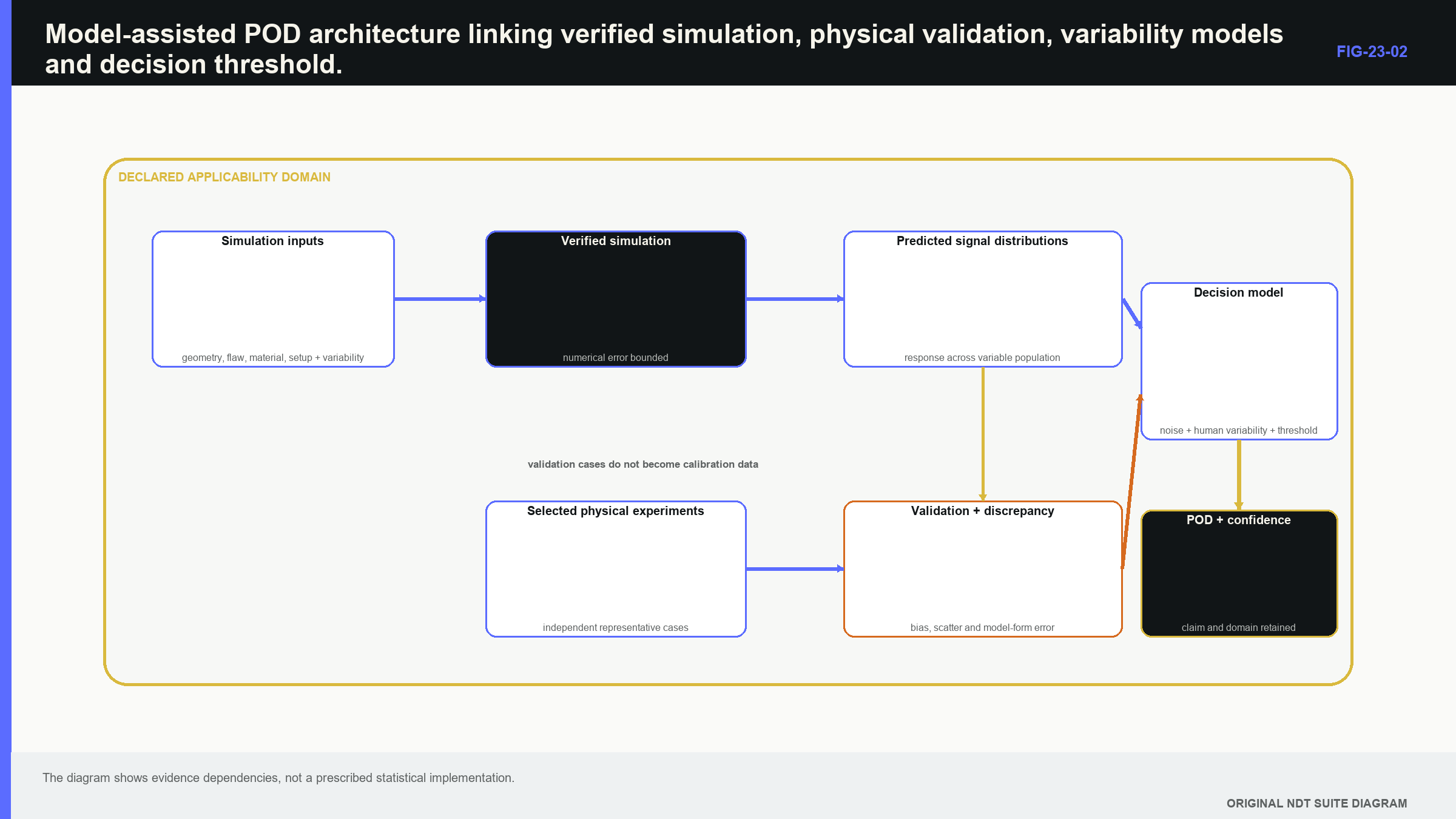
Matching amplitude from one normal flat-bottom hole does not validate skewed crack responses in anisotropic welds; sensitivity analysis should identify which inputs need physical coverage. Tuning uncertain inputs until one comparison looks perfect can hide model discrepancy and weaken prediction. Federal Railroad Administration work on ultrasonic rail inspection demonstrates the integration of physical and simulation programmes. [R035] Its transferable lesson is that simulation extends a defined evidence programme; it does not convert sparse validation into universal performance.
The same programme provides a useful reminder that validation points, noise assumptions and physical trials remain part of the MAPOD architecture rather than optional decoration around the simulation. [R035] Formal probability integration, probability-updating alternatives and model-discrepancy treatment are reserved for Chapter 64.9 and Chapters 78.6 to 78.8.
23.10 Sizing reliability is a different claim
Detection reliability does not establish sizing accuracy; a sizing study needs bias, spread, outliers, dependence on true size, failure-to-size rate and coverage of any reported uncertainty. A method can detect small flaws reliably while overestimating height. It can size larger clean targets well while failing to resolve smaller tips.
| Worked example · Sizing bias across a tested range WE-23-02 Given: Known heights are 3, 5, 7, 9 and 11 mm. Mean measured values are 4.0, 6.1, 8.0, 10.2 and 12.1 mm. Find: Mean bias across these five points. Steps: Errors are +1.0, +1.1, +1.0, +1.2 and +1.1 mm. Their mean is 5.4/5 = 1.08 mm. Answer: Observed mean bias is approximately +1.1 mm over the tested 3 mm to 11 mm range. Technical implication: A correction is defensible only if the bias is stable and representative, and its own uncertainty is carried. Common mistake: Five mean points do not establish behaviour outside the range or reveal individual outliers and failed measurements. |
|---|
Mean bias can look acceptable when large positive and negative errors cancel; residual plots should show spread and size dependence. Failure cases must remain in the dataset. Replacing a censored result such as “greater than 20 mm” with 20 mm creates bias. Analysing only successfully sized targets overstates conditional performance. Measurement uncertainty terminology and the separation of repeatability and model contributions are supported by the metrology references. [R031] [R032] Chapter 78 extends these concepts with variance components, nonlinear propagation and decision uncertainty.
23.11 Technical decision case: releasing a reliability statement
Suppose the running technique from Chapter 22 is tested on several representative specimens by multiple operators; outcomes span the target-size transition, unflawed regions are included, and the call rule is fixed before scoring. A fitted POD model and lower bound are reported only within the tested domain. False-call evidence and operator grouping remain visible. A separate sizing study shows positive height bias and several unresolved tips.
The release can support detection reliability for the declared ferritic weld, flaw and operator population when diagnostics are adequate; it can report the tested range and confidence method. It should not claim the same POD for austenitic repairs, new software thresholds or unseen target orientations. It should also keep sizing outside the detection claim until the sizing evidence supports a separate statement. A usable reliability statement names the system, population, flaw measure, operators, equipment, threshold, association rule, study design, statistical model, confidence method, tested range, exclusions and false-call result; it shows observations with curves. Missing data and deviations remain visible.
The purpose is not the largest percentage; it is a result that another technical decision-maker can interpret and challenge. A vague “90% POD” remains marketing-shaped fog, even when the fog has acquired a confidence-coloured border.
23.12 Formal depth and the Part VIII handoff
At Level 3, the learner should calculate descriptive results, read fitted reliability outputs and judge study support. The mathematical derivations are staged later:
- Chapter 64.9 introduces probability models and Bayesian updating, which revises probability descriptions as evidence arrives.
- Chapter 78.6 develops POD as a metrology and reliability problem.
- Chapter 78.7 develops model-assisted POD.
- Chapter 78.8 connects thresholds, false calls and consequences.
- Chapters 78.12, 78.13 and 78.17 develop variance components, model diagnostics and clustered trials.
- Chapter 78.18 treats sample planning and information.
The separation is deliberate; Part III teaches what the statistics mean and how they support a technical claim before Part VIII derives and extends the models.
In plain words
- Nineteen detections in twenty trials is an observed fraction, not a population guarantee.
- POD belongs to a defined system, target population and decision rule.
- A confidence bound expresses finite-study uncertainty around a fitted model.
- Hit-miss and signal-response studies retain different information and assumptions.
- False calls must be assessed with a meaningful denominator and realistic unflawed regions.
- Repeated scans sharing flaws, people or specimens are not automatically independent.
- MAPOD extends physical evidence only inside a verified and validated model domain.
- Detection reliability and sizing reliability require separate evidence.
Key terms
- Detection fraction: observed detections divided by eligible trials.
- POD: modelled probability of detection for a declared system and population.
- Confidence bound: conservative boundary reflecting sampling uncertainty.
- Hit-miss data: binary trial outcomes.
- Signal-response data: continuous response with a declared threshold.
- False call: detection decision in an unflawed decision region.
- Clustering: shared factors that make outcomes dependent.
- MAPOD: physical and simulation evidence combined for POD estimation.
Key relationships
- p_hat = k/n: observed fraction describes the study data only.
- POD(a) = 1/[1 + exp(-(beta_0 + beta_1 a))]: logistic model relates detection probability to declared flaw size under its assumptions.
- threshold down -> hits often up and false calls often up: operating point is a consequence-informed trade-off.
- qualification evidence != routine condition check: each answers a different reliability question.
Common mix-ups
- Observed detection fraction is not the same as population POD.
- A fitted POD curve is not its lower confidence bound.
- Many repeated scans are not many independent flaws.
- A reference echo does not maintain population evidence by itself.
- Good detection performance does not prove unbiased sizing.
Bridge to Chapter 24
Reliability transfer depends on the production population resembling the study population; chapter 24 examines cases where that transfer fails because material, geometry, temperature or access breaks the simple propagation assumptions. Its first diagnostic step identifies which assumption failed before selecting another frequency, mode, model or method.
Sources and further study
- [R031]
- [R032]
- [R033]
- [R034]
- [R035]
- [R052]
Study and revision only. This is not an approved inspection procedure, acceptance criterion or qualification.