
CHAPTER 24 · Ultrasonics Level 3
Difficult Materials, Geometry and Honest Capability
In this chapter · 21 sections
Why this matters
A Level 2 technician can establish a reference and complete a scan while still lacking useful evidence in part of a component; a coarse casting may show no stable far surface. An austenitic weld may move the beam away from its isotropic location. A curved surface may defocus a previously narrow field. A composite may return strong interface echoes while hiding deeper damage. Level 3 does not respond by adding gain until the display glows with optimism. It identifies the failed simple assumption, chooses evidence that tests the failure mechanism and reports any remaining capability gap.
What you already need
- The homogeneous, isotropic ray and beam models used in Level 2.
- Wavelength, attenuation, refraction, mode conversion and target orientation.
- Representative-reference and signal-to-noise concepts.
- The model-selection and field-characterisation ideas from Chapters 19 and 20.
- The bounded claim and applicability-domain concepts from Chapters 22 and 23.
What you will learn
- Diagnose the simple assumption that failed in a difficult examination.
- Compare absorption, scattering, redirection, defocusing and coupling symptoms.
- Select evidence for castings, directional welds, curved parts and composites.
- Explain temperature and mechanisation as fields and coordinate problems.
- Use complementary methods to answer a named unresolved question.
- Produce a capability map that separates detection, location, sizing and no-assessment regions.
Words you will meet
- Heterogeneous: having properties that vary from place to place.
- Random medium: material represented by spatially varying properties and statistics.
- Coherent field: part of the field retaining predictable phase relationship.
- Speckle: spatial interference pattern produced by many scattering contributions.
- Defocusing: spreading of field energy away from the intended concentration.
- Homogenisation: replacement of fine structure by effective average properties.
- Registration: mapping between scanner, component and material coordinates.
- Thermal gradient: change in temperature with position.
- Complementary evidence: evidence from a different interaction or coverage route.
- Capability map: spatial statement of which outputs are supported in each region.
Depth guide for this chapter
- Understand here: diagnostic symptoms, material cases, complementary evidence and capability limits.
- Calculate here: wavelength-to-structure scale, coordinate bias and simple path-loss comparisons.
- Derive later: random-media statistics, anisotropic solvers, coordinate transformations and full temperature-field models continue in Chapters 65, 66, 70 and 76.
24.1 Diagnose the failed assumption first
An examination becomes difficult when ordinary assumptions fail enough to threaten the required output; those assumptions include homogeneous material, direction-independent velocity, smooth accessible surface, known geometry, stable coupling, adequate coherent response and one identifiable path. Common symptoms include:
- a beam peak displaced from its predicted position;
- different velocities or locations from opposite directions;
- rapidly changing response over a small probe movement;
- loss of high-frequency content with path;
- no stable far-surface or reference response;
- strong geometry echoes combined with uncertain target access;
- split modes or several plausible arrival paths;
- coupling that changes as a probe rocks over curvature.
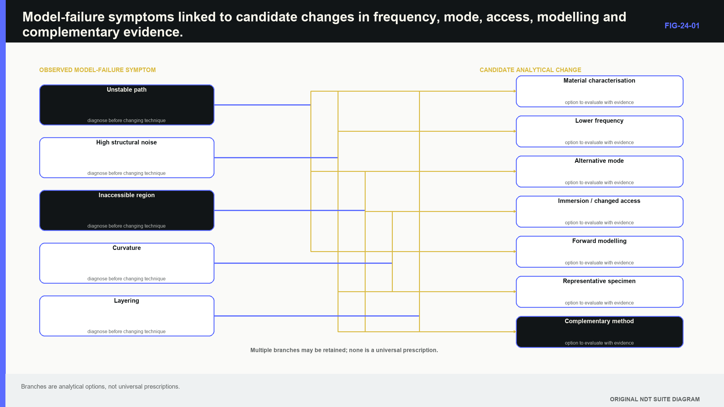
The next observation should divide causes; a mapped peak that shifts laterally with little loss points toward redirection. A stable direction with progressive high-frequency loss points toward absorption or scattering. A response that changes sharply with small surface movement can indicate coupling or speckle. An electrical reference that remains stable removes much of the instrument receiver from the leading hypothesis set. One peak amplitude rarely distinguishes the mechanism; the diagnostic aim is not perfect scientific identification before progress. It is enough evidence to choose the next field, frequency, mode, access or model intelligently.
The figure below organises those choices; notice that each branch begins from an observed capability problem rather than from a favourite special technique.
24.2 Case one: a coarse-grained casting
Cast components can contain large, variable grains and complicated surfaces; each grain can have a different crystallographic orientation and local stiffness. The travelling field accumulates phase variation, coherent response falls and structural backscatter grows. Geometry can focus or shadow the field at the same time. Lower frequency often improves penetration because wavelength grows relative to grain scale; the trade-off is a longer pulse, a wider field and reduced separation. A larger aperture can restore some directivity and energy, while increasing the coupling footprint and near-field complexity.
The scale comparison can be expressed as follows.
| (24.1) Wavelength-to-structure ratio · EQ-24-02 Where: eta = dimensionless scale ratio; lambda = wavelength (m); d_structure = representative heterogeneity dimension (m) Model limits: one representative scale; does not by itself predict scattering magnitude |
|---|
The relationship supports initial frequency comparison; large eta makes an effective-medium starting model more plausible. It does not calculate scattering from grain size alone because grain shape, texture, elastic contrast and spatial correlation also matter.
| Worked example · Comparing wavelength with grain scale WE-24-02 Given: Example longitudinal velocity is 5,800 m/s, and representative grain scale is 1.0 mm. Compare 5 MHz and 1 MHz. Find: Wavelength and wavelength-to-grain ratio at each frequency. Steps: At 5 MHz, lambda = 5800/(5 x 10^6) = 1.16 mm, giving eta = 1.16. At 1 MHz, lambda = 5.8 mm, giving eta = 5.8. Answer: The 5 MHz wavelength is comparable with grain scale, while the 1 MHz wavelength is several times larger. Technical implication: Stronger scattering risk at 5 MHz is plausible. Physical trials still determine whether the lower-frequency loss of resolution is acceptable. Common mistake: Treating the ratio as a direct formula for signal-to-noise ignores field, elastic contrast and target response. |
|---|
Reference targets must lie behind representative material paths; a strong near-surface response does not prove capability at depth. A fine-grained wrought reference can show instrument condition but cannot demonstrate penetration through the casting. Cast-material field studies reinforce that deep capability follows the characterised aperture and actual propagation path, not the presence of a convenient shallow response. [R011] [R012]
Low-frequency array and field studies in cast austenitic stainless components show that aperture, frequency, material path and scan geometry must be characterised for the application. [R011] [R012] They do not define one universal casting probe. Post-acquisition averaging also needs care; independent spatial samples can reduce random components, while correlated samples mainly smooth the same speckle. A large aperture and spatial averaging can both suppress a local target or hide shadowed regions. More averaged data are not automatically more independent evidence.
24.3 Case two: an austenitic or dissimilar-metal weld
Austenitic weld metal can contain oriented dendrites whose direction changes with pass and fusion geometry; wave speed, polarisation and attenuation become directional. Energy can skew, broaden or split into quasi-modes. Cladding and dissimilar interfaces add path changes and reflection. The practical symptom can be a repeatable echo that plots in the wrong place, or a target that appears from one direction and disappears from another; one average velocity may fit one reference and misplace a different path. Increasing gain at the isotropic predicted coordinate cannot restore coverage when energy travelled elsewhere.
| Worked example · Distinguishing attenuation from beam redirection WE-24-01 Given: In an anisotropic weld, a nominal beam gives a weak target response at the isotropic predicted position. A field scan finds peak energy 9 mm lateral to that position and only 2 dB below the peak in parent material. Find: The leading explanation for the missing response at the predicted position. Steps: Compare total peak loss with spatial movement. The measured field retains nearly the same peak level but reaches another coordinate. Answer: Beam redirection or skew is the leading cause rather than severe overall attenuation. Technical implication: The path model or probe arrangement must represent actual energy direction. Gain at the wrong position does not create coverage. Common mistake: Comparing amplitude only at the predicted point confuses moved energy with lost energy. |
|---|
Longitudinal modes can sometimes retain more useful energy than shear modes in these welds, but that tendency is not universal; frequency, texture direction, target orientation and access remain part of the case. Multiple sides and modes can add orientation coverage and reveal inconsistent location. Macrostructure-informed ray or full-wave models can generate candidate paths; their value depends on actual orientation and elastic inputs. A generic weld sketch makes the result a hypothesis rather than a validated field. Physical mapping and representative targets remain necessary. United States Department of Energy (DOE) work documents the importance of anisotropy and scattering in austenitic weld inspection. [R008]
That work also supports treating direction-dependent propagation as an application variable that must be demonstrated rather than a small correction hidden inside an isotropic setup. [R008]
| Worked example · Separating velocity and direction effects in an anisotropic path WE-24-03 Given: An isotropic model uses 5,900 m/s and 45 degrees for a 50 microsecond one-way arrival. Field evidence indicates an energy direction of 51 degrees and effective group speed of 5,650 m/s. Find: Modelled and revised endpoints from the same arrival time. Steps: Model path is 5900 x 50 x 10^-6 = 295 mm; coordinates are x = z = 208.6 mm. Revised path is 5650 x 50 x 10^-6 = 282.5 mm; coordinates are x = 282.5 sin51 = 219.5 mm and z = 282.5 cos51 = 177.8 mm. Answer: Relative to the isotropic model, the revised endpoint moves about +10.9 mm laterally and -30.8 mm in depth. Technical implication: Correcting velocity alone cannot correct direction. Precise timing can coexist with substantial location bias. Common mistake: Applying a scalar velocity correction while retaining the isotropic angle leaves the main spatial error unresolved. |
|---|
At Level 3, the calculation uses measured speed and direction; deriving those quantities from stiffness and texture belongs to Chapters 65.14, 65.18 and 66.1 to 66.8.
24.4 Case three: curvature and restricted access
Curvature changes the local surface normal across a finite probe footprint; a convex surface can spread the transmitted field. A concave surface can focus it or form a concentrated region. The probe can rock, creating variable coupling and entry position. Small cylinders can support repeated circumferential paths. Nozzles and branches vary surface normal and wall thickness in more than one plane; a two-dimensional cross-section can explain one local path while overstating volumetric coverage. Useful remedies include contoured wedges, immersion, smaller apertures, encoded position and three-dimensional geometry models. Each remedy introduces its own variables.
A contoured wedge matches only the curvature and orientation for which it was made; wear, lift-off and rotation reintroduce mismatch. Immersion adds water path, surface registration and interface echoes. A robot improves repeatability while adding coordinate calibration, backlash, path-following and missed-data risks. Three coordinate systems should remain visible; scanner coordinates describe machine motion. Component-surface coordinates describe the part. Material coordinates describe acoustic position inside the component. Registration maps one system into the next. A precise encoder cannot repair a wrong surface model.
Coordinate uncertainty should expand where geometry is poorly known; coverage can be represented by a three-dimensional field envelope across plausible surface and registration variation. This is more defensible than projecting one central ray through a nominal drawing.
24.5 Case four: a layered composite or bond
Composite laminates combine directional plies, interfaces and repeated structure; ply direction controls phase and energy behaviour. Interfaces create reverberation and mode conversion. Porosity and fibre waviness produce distributed scattering. A shallow delamination can shadow damage below it. Homogenisation can be reasonable when wavelength is much larger than the repeating architecture; as wavelength approaches ply or cell scale, direction, dispersion and mode conversion become more visible. NASA composite resources emphasise matching ultrasonic physics to architecture, geometry, wavelength and damage type. [R003] Analytical composite ultrasonics also shows that energy direction can differ from phase direction and that effective-medium assumptions have scale limits. [R006]
Different damage types produce overlapping signals; delamination behaves like an interface but changes with contact, fluid ingress and incidence. Porosity produces distributed scattering and loss. Impact damage can combine delamination, matrix cracking and fibre breakage. One amplitude image rarely classifies all mechanisms uniquely. Composite guidance and analytical treatments both reinforce the need to connect architecture and wavelength to the claimed damage response. [R003] [R006]
Bond evaluation illustrates the evidence boundary; ultrasound can measure reflection, transmission, resonance or stiffness-related behaviour at an interface. It does not measure future adhesive strength universally. A weak interface echo can arise from good impedance continuity, a very thin layer, resonance, incidence or poor coupling. A strength claim needs a validated relationship for the particular materials, geometry and degradation mechanism.
24.6 High temperature is a field problem
Temperature affects component and wedge velocity, attenuation, couplant and transducer behaviour; a thermal gradient means temperature changes along the path. One correction temperature cannot represent every part of the wave journey. For a defined ray in a spatially varying speed field, travel time is expressed as:
| (24.2) Travel time through a spatially varying speed field · EQ-24-01 Where: t = transit time (s); ds = differential path length (m); c(s) = local group speed along the path (m/s) Model limits: a defined ray path and sufficiently gradual variation for ray treatment |
|---|
The equation states that small path segments contribute according to local slowness; it supports understanding of why an average temperature may bias time. If the gradient also bends the ray, path and speed must be solved together. Performing that integration or coupled ray solution is a Part VIII task in Chapters 64.3, 66.12 and 70. Delay lines and waveguides can protect active material while adding modes, reflections and temperature-dependent delay; a stable reference near the surface may not represent the deeper temperature field. The measurement system should separate reversible thermal change from permanent transducer or couplant damage.
24.7 Immersion and mechanised acquisition
Immersion provides controlled coupling, stand-off, focusing and encoded scanning; it also creates a strong water-component interface, refraction sensitivity, alignment requirements and water-path multiples. Raster pitch must represent the smallest task-relevant field and target scale. Mechanisation improves positional repeatability but does not correct the wrong field; it adds encoder direction, backlash, trigger completeness and registration. Chapter 21 showed that missing acquisitions can create hidden spatial gaps. In difficult geometry, the coordinate model is part of acoustic capability rather than an administrative afterthought.
An automated path should preserve evidence of actual pose, contact or water path and acquisition count; a visually complete image can be reconstructed from data that never sampled part of the intended surface. The capability claim follows measured coverage, not the smoothness of the motion animation.
24.8 Complementary methods answer named gaps
A complementary method is useful when it observes a different physical feature or reaches an unsupported region; more views from the same flawed path may add correlation without adding new evidence. Time-of-flight diffraction uses separated transmitter and receiver paths and diffracted energy from discontinuity extremities; it can provide time-based height evidence where pulse-echo face response is strongly directional. Entry and far-surface dead zones, geometry and signal identity still limit it.
Guided-wave methods use dispersive modes constrained by plates, pipes or rails to screen long distances; they trade local detail for range and depend on frequency-thickness product, mode selection, attachments and environment. Benchmarking work shows that solver agreement on one problem does not establish broad validity. [R036] The same benchmarking principle applies when a guided-wave model is transferred to another geometry or boundary condition; agreement must be re-established inside the new use domain. [R036]
Electromagnetic acoustic transducers, laser ultrasonics and air-coupled systems can reduce liquid coupling, while introducing lift-off, conversion-efficiency, optical or signal-to-noise constraints; chapter 75 provides the engineering treatment. Surface methods can confirm surface breaking. Radiography can contribute projected volumetric evidence. Through-transmission can reveal loss of continuity when pulse-echo geometry remains ambiguous. The choice follows the unresolved question; beam skew needs a different path or field measurement. Tip identity needs independent extremity or orientation evidence. An unexamined volume needs a method whose field enters that volume. Complementary does not mean automatically superior or fully independent.
24.9 Technical decision case: incomplete casting penetration
Suppose a low-frequency probe provides a stable far-surface response across 70% of a casting; the remaining 30% shows strong structural noise and no stable deep reference. No discrete indication is resolved there. The supported result is not “no indications throughout.” Detection capability is demonstrated only where representative deep response and coverage remain adequate; the unresolved region may be challenged with another frequency, aperture, mode, surface, representative target or complementary method. If none restores evidence, the limitation belongs in the result and the downstream decision.
This case separates three decisions; the 70% region can support its demonstrated output. The noisy region cannot support an absence conclusion. The entire component may still receive an engineering disposition that combines the bounded ultrasonic result with other evidence. Level 3 supplies the capability map; it does not erase the map to make the report simpler.
24.10 Capability maps and evidence boundaries
A capability map divides the component into regions supported for different outputs; one area may support detection and location but not sizing. A second may have penetration but poor orientation response. A third may remain inaccessible or acoustically unresolved. Each region should trace to evidence: representative reference response, measured field, material characterisation, geometry registration, access and uncertainty; boundaries can be bands rather than sharp lines. If capability depends strongly on target orientation, the map needs an orientation dimension or separate views.
Incomplete coverage is a valid engineering result; it identifies where the measurement system cannot support a conclusion and allows another method, changed access or structural assessment to address the remaining uncertainty. The unacceptable shortcut is converting absence of interpretable evidence into absence of a discontinuity. The advanced material architecture and tailored inspection treatment continues in Chapter 76; random propagation, stochastic fields and model discrepancy continue in Chapters 66.10 to 66.20. Numerical modelling and validation continue in Chapter 70.
In plain words
- A difficult examination is one where simple assumptions fail enough to threaten the decision.
- Lost amplitude can arise from absorption, scattering, redirection, defocusing, coupling or recovery.
- Coarse grains require frequency and field choices based on representative material paths.
- Directional welds can produce precise times and wrong coordinates.
- Curvature creates acoustic and coordinate errors that an encoder alone cannot correct.
- Composite response depends on architecture, direction, interfaces and damage type.
- Complementary methods are chosen to answer a named unsupported question.
- A capability gap should be mapped and reported rather than converted into a soundness claim.
Key terms
- Heterogeneous: varying in material properties with position.
- Random medium: spatially varying material represented statistically.
- Coherent field: field component retaining predictable phase relation.
- Speckle: interference pattern from many scattering paths.
- Defocusing: field spreading away from the intended region.
- Homogenisation: use of effective properties in place of fine structure.
- Registration: transformation between scanner, component and material coordinates.
- Capability map: supported outputs assigned to component regions.
Key relationships
- eta = lambda/d_structure: wavelength-to-structure scale guides the starting propagation model.
- t = integral ds/c(s): a varying speed field contributes local travel delay along the path.
- diagnostic symptom -> discriminating observation -> model or technique change: causal diagnosis guides evidence.
- available data != demonstrated capability: interpretable reference and target response define the supported region.
Common mix-ups
- More gain is not more penetration.
- A missing echo is not proof of no discontinuity.
- Lower frequency is not automatically an adequate technique.
- A simulation is not qualification.
- Encoded motion does not correct a wrong acoustic field or coordinate model.
Bridge to Chapter 25
Chapter 24 ended with evidence that can be incomplete, contradictory or supported only for selected regions; chapter 25 carries those boundaries into sizing and integrity communication. It begins by defining crack tips, ligament and sizing bias in plain language before introducing structural-assessment context.
Sources and further study
- [R003]
- [R006]
- [R008]
- [R011]
- [R012]
- [R036]
Study and revision only. This is not an approved inspection procedure, acceptance criterion or qualification.