
CHAPTER 4 · FMC / TFM / PCI Level 2
Signals, Phase and Matrix Data Literacy
In this chapter · 15 sections
Learning outcomes
After completing this chapter, the learner should be able to:
identify transmitter and receiver axes in an FMC matrix;
distinguish diagonal self-pairs from off-diagonal pitch-catch pairs;
calculate nominal full-matrix and reciprocal unique-pair counts;
explain what reciprocity can and cannot justify;
locate a selected A-scan within an FMC dataset;
distinguish fixed-pair time traces from fixed-time matrix slices;
recognise timing, clipping, noise and missing-channel patterns; and
perform a structured dataset audit before reconstruction.
Crossover map
| Familiar evidence | Matrix-data equivalent | New question to ask |
|---|---|---|
| One pulse-echo A-scan | One diagonal matrix cell | Which transmitter and receiver produced it? |
| Pitch-catch trace | One off-diagonal cell | What are the separate transmit and receive paths? |
| Element check | Row, column and cell health patterns | Is the fault transmit-side, receive-side or isolated? |
| Time base | Sample count, interval and acquisition origin | Is sample zero physically defined? |
| RF waveform | Pair-specific signed time series | Are phase and polarity preserved? |
| Encoded PAUT frame | A full matrix at each scan position | Are matrices complete and correctly position-linked? |
| Stored image | Raw matrix plus metadata and derived images | Can the image be independently reconstructed? |
The transmit-receive matrix
An FMC acquisition can be represented as a table. Rows identify transmitting elements. Columns identify receiving elements. The cell in transmitter row i and receiver column j contains the A-scan recorded for that ordered pair. This book writes that trace as Aij.
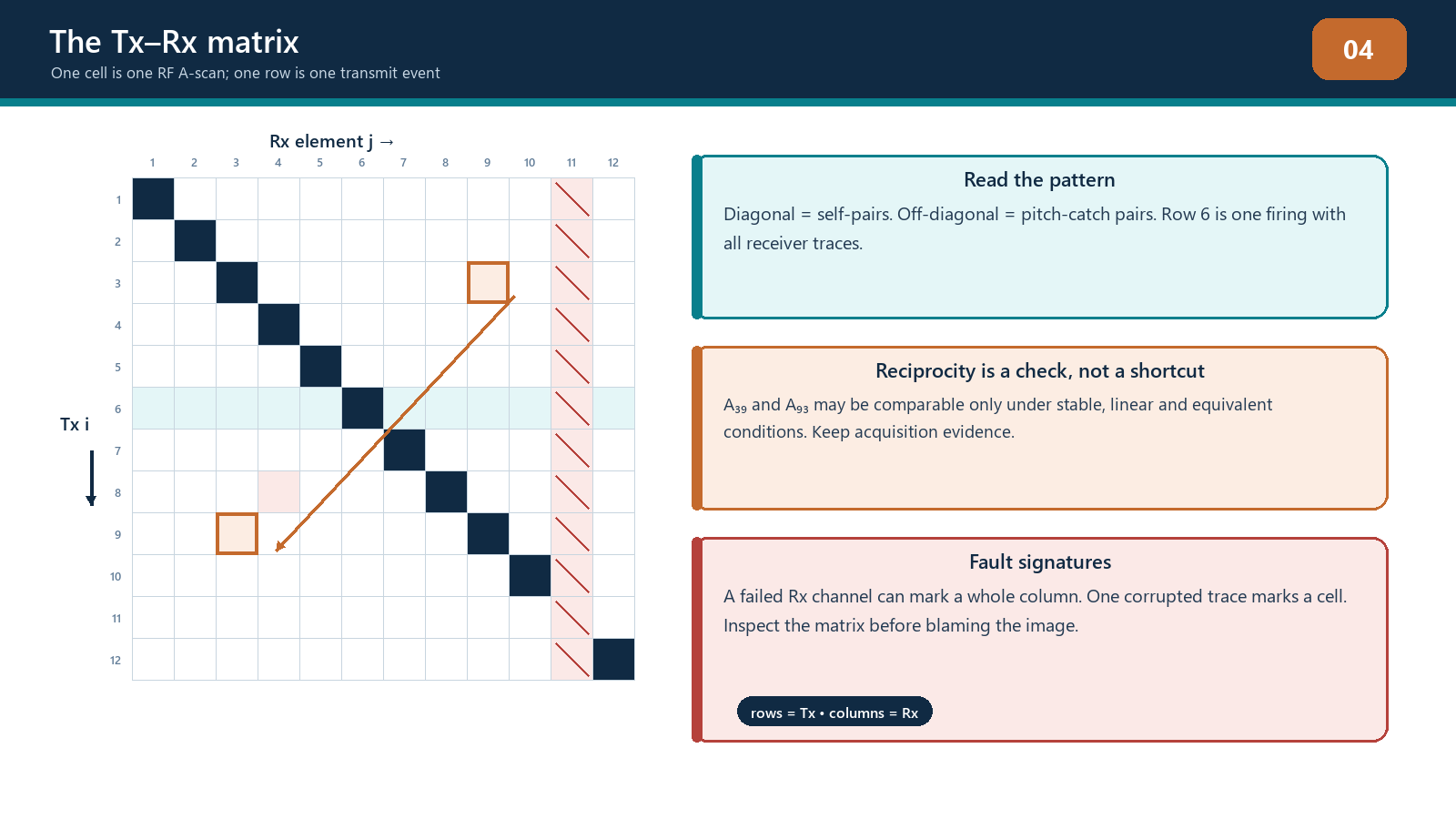
The main diagonal contains cells for which transmitter and receiver are the same element. These are self-pairs and resemble conventional pulse-echo geometry. Off-diagonal cells use different transmit and receive elements. Their total path is the transmitter-to-interaction leg plus the interaction-to-receiver leg.
One complete row normally represents one transmit event recorded on all selected receivers. One complete column represents one receiver's signals across all transmit events. These patterns are useful for fault diagnosis:
a weak or missing row can indicate a transmitter, pulser, sequence or coupling problem associated with that element;
a weak or missing column can indicate a receiver-channel problem;
a weak row and column associated with one physical element can indicate element, wiring or contact problems; and
one isolated cell can indicate a trace-specific acquisition, transfer or file defect.
The pattern suggests a cause; it does not prove it. Confirm the channel assignment, sequence, probe wiring and repeatability before replacing equipment or excluding data.
Counting pair traces
If NTx transmitters and NRx receivers are used and every ordered combination is recorded, the nominal number of traces at one acquisition position is:
N_traces = N_tx x N_rx
For a square 64-element sequence with all elements transmitting and receiving, this is 4,096 pair traces at each position. If 1,000 encoded positions are acquired, the dataset contains more than four million pair traces before considering sample count or metadata.
Under linear reciprocal conditions, the acoustic transfer from element i to element j can be comparable with the transfer from j to i. If the diagonal is included and each reciprocal pair is counted only once, the number of unique unordered pairs for N elements is:
N_unique = N(N + 1) / 2 (only when qualified reciprocity assumptions apply)
For N = 64, that count is 2,080. This arithmetic does not authorise deletion of the other half of a production matrix. Reciprocity depends on equivalent propagation, stable coupling, linear response, consistent electronics and timing. Ordered traces can differ because the transmit and receive chains do different jobs. The intended reduced acquisition must be identified and demonstrated.
Reciprocity as a diagnostic
Reciprocal pairs provide a valuable comparison. If Aij and Aji differ substantially in arrival time, phase form or usable frequency content under stable conditions, investigate:
element or channel timing offsets;
different transmit and receive bandwidths;
probe wiring or element-map error;
unstable coupling between sequence events;
motion during acquisition;
clipping or low signal-to-noise ratio;
non-linear response; and
file corruption or trace misassignment.
Exact waveform equality is not required. A transmitting element is driven by a pulser while a receiving element is connected to a receiver chain, and the reverse event occurs at a different time in the sequence. Compare the features relevant to the technique rather than demanding identical sample values.
Reciprocity can also be used to test data consistency before TFM. Broad systematic disagreement warns that pair summation may not behave as expected. It does not automatically mean every disagreement is a defect in the instrument; the experimental conditions and expected tolerance must be defined.
The A-scan inside each cell
Every matrix cell contains a sampled waveform over time. A useful pair A-scan may include:
a pre-trigger or baseline region;
electrical cross-talk or initial-pulse response;
wedge or entry-surface activity;
target, geometry or backwall response packets;
reverberations or mode-converted arrivals; and
a final region in which no relevant path should arrive.
The technician should identify which regions are expected for the selected pair and component. A response occurring at the correct pulse-echo depth on a diagonal trace may occur at a later time on a widely separated off-diagonal trace because the total path is longer. Conversely, an electronic event fixed at the same sample across most pairs may not represent a material reflector.
Trace amplitude should be checked in signed RF form when phase or summation is important. Rectification or envelope processing can hide clipping asymmetry, polarity reversal and waveform alignment. If only processed traces are retained, record that limitation.
From a matrix to a data cube
A two-dimensional matrix identifies transmitter and receiver. Each cell extends along a third dimension: sample index or time. At one encoded position, the data can therefore be imagined as a transmit-by-receive-by-time block. During an encoded scan, position adds another dimension.
Two views of this structure are particularly useful:
a fixed-pair trace, which follows one cell through time and looks like an A-scan; and
a fixed-time slice, which shows the instantaneous signed value for every pair at one selected sample.
A TFM pixel does not copy one cell or one fixed-time slice. It calculates a different predicted time for each usable pair, extracts or interpolates samples at those times and combines them. The collection of samples used for one pixel therefore cuts through the data cube along a model-defined surface.
This distinction explains why a bright response can disappear when velocity or geometry changes. The raw traces remain the same, but the reconstruction samples them at different times.
Phase literacy for matrix data
Phase describes position within an oscillation. For a narrow packet, similar physical interactions recorded through different pairs can contain corresponding positive and negative lobes at pair-dependent arrival times. TFM aligns the predicted arrival regions so contributions reinforce. PCI examines phase agreement using its documented processing.
Three cautions are essential:
Time alignment and phase agreement are related but not identical. A small timing error can shift a sample into a different phase lobe even when the envelope peak remains nearby.
Phase depends on retained frequency content and processing. Filtering, resampling, analytic-signal conversion and polarity handling can change the representation.
Noise can be coherent. Electrical cross-talk, reverberation and geometry responses can repeat consistently across pairs and produce structured image response.
The correct question is not simply Is the phase coherent? It is Is the phase coherence consistent with the declared acoustic path and component geometry, and is there corroborating evidence?
Timing, interpolation and the sample grid
Travel-time calculations rarely land exactly on a stored sample. Reconstruction software may select the nearest sample or interpolate between samples. The method can affect amplitude fidelity, phase behaviour and computation time. It should be documented where it is configurable or material to qualification.
Channel timing should be stable to a small fraction of the pulse period for reliable coherent summation. Element-to-element timing offsets can broaden point responses or reduce coherence. Wedge delay and acquisition origin affect all path calculations, while a single channel delay can create a structured row/column problem.
Increasing the sampling frequency can reduce time-grid spacing but does not restore bandwidth absent from the analogue signal. Digital interpolation can make timing estimates smoother but does not add new independent acoustic observations.
Dataset metadata
A matrix without context is not an examination record. At minimum, preserve:
instrument, software and firmware identification;
probe, wedge and element-map identity;
transmit and receive selections and sequence order;
pulser, receiver, filter and digitisation settings;
sampling frequency, sample count, time origin and delays;
component, material, velocities and geometry model;
coordinate origin, array orientation and encoded direction;
acquisition position, increment and encoder scale;
coupling and surface condition notes;
reconstruction recipes and derived-image versions; and
calibration, verification and change history.
If raw data are exported, confirm whether filtering, compression, rectification, pair reduction or proprietary conversion occurred. The word raw is frequently optimistic.
Matrix health signatures
Dead or weak element
A physical element problem can affect its transmit row and receive column. The pattern may vary because transmit and receive sensitivity are not identical. Confirm using the approved element check and a stable target.
Receiver-chain fault
A weak column across many transmitters suggests a receive-side issue. Compare neighbouring columns and repeat under stable coupling.
Transmit-sequence fault
A weak row across receivers suggests the corresponding transmit event was absent or abnormal. Check the pulser selection, firing sequence and element map.
Saturation
Clipped traces show flattened positive or negative peaks and lost waveform shape. Saturation can be limited to strong diagonal or near-surface pairs, so an overall image may not reveal it clearly.
Cross-talk and fixed-time interference
An electrical event occurring at a similar time across rows or columns can form a line or arc after reconstruction. Compare behaviour when coupling or the component path changes.
Position dropout
In encoded data, one entire matrix or a group of matrices can be missing, repeated or assigned to the wrong coordinate. Image discontinuity across scan position may be an encoder/file problem rather than a physical feature.
Field workflow: audit before reconstructing
Verify file identity, component, probe, wedge and acquisition revision.
Confirm matrix dimensions match the declared transmit and receive selections.
Check sample count, sample interval, time origin and signal representation.
Inspect representative diagonal, near off-diagonal and wide off-diagonal traces.
Review row and column health maps for weak, missing or clipped channels.
Compare selected reciprocal pairs under the approved diagnostic tolerance.
Check encoded position count, increment, direction and discontinuities.
Confirm raw data and required metadata are retained.
Record exclusions or corrections before reconstruction.
Stop if the remaining data have not been demonstrated as sufficient for the intended method.
Practical 4 - Audit an FMC matrix
Objective
Identify dataset structure and diagnose deliberate data-integrity faults before viewing the final reconstruction.
Resources
a documented teaching dataset with known matrix dimensions;
matrix-view and RF-trace tools;
a truth record retained by the instructor; and
a blank audit form.
Method
Record the transmitter, receiver, sample and position dimensions.
Calculate the expected full trace count per position and reciprocal unique-pair count.
Identify the diagonal, one transmit row, one receiver column and three reciprocal pairs.
Inspect RF traces from self, near pitch-catch and wide pitch-catch geometries.
Locate deliberate weak, missing, clipped or timing-shifted traces.
Classify each pattern as likely transmit, receive, element, isolated trace or position fault.
Compare selected reciprocal pairs and state whether differences are technically significant.
Decide whether to accept, exclude, reacquire or escalate, and state the evidence basis.
Required evidence
labelled matrix map;
pair-count calculations;
six annotated RF traces;
fault table with symptom, hypothesis, confirming test and action; and
signed dataset disposition.
Stop rules
Do not reconstruct until the transmitter/receiver convention, sample origin and signal representation are known. Stop if matrix reduction or missing traces are not covered by the teaching technique. Do not repair raw data by copying neighbouring traces.
Successful completion
The learner locates all seeded faults, distinguishes pattern evidence from proof, and makes a conservative data disposition consistent with the declared technique.
Common traps
Assuming rows and columns use the same convention on every system. Verify whether rows are transmitters before diagnosing patterns.
Treating reciprocal pairs as identical by definition. Reciprocity is a physical expectation under stated conditions, not permission to ignore measured differences.
Inspecting only diagonal traces. TFM relies heavily on off-diagonal pair geometry.
Calling processed envelope data raw RF. Confirm sign, filtering and conversion history.
Ignoring isolated saturation. A clean final image can hide clipped contributing traces.
Using matrix symmetry to fill missing data. Any reduced or reconstructed dataset needs controlled validation.
Chapter summary
An FMC matrix is an organised set of pair-specific A-scans. Rows normally represent transmitters, columns receivers and the diagonal contains self-pairs. Time extends every cell into a third data dimension, while scan position can add a fourth. Trace counts grow rapidly with array size. Reciprocity supports comparison and some controlled acquisition strategies but is not an unconditional equality. Matrix literacy lets the technician detect row, column, cell, timing and position faults before reconstruction hides them inside an image.

Study and revision only. This is not an approved inspection procedure, acceptance criterion or qualification.