
CHAPTER 15 · Ultrasonics Level 2
Read the Weld Before Reading the Echo
In this chapter · 20 sections
Why this matters
A strong echo close to the root is not automatically a root crack. It could come from the root profile, mismatch, backing, lack of penetration, a fusion-face reflector or a path that changed wave mode. The screen reports returned sound; it does not name the cause. Reliable weld interpretation starts with the actual joint and turns probe movement into a series of small tests. This chapter gives a practical sequence for doing that before the deeper interpretation methods of Level 3.
What you already need
- Basic weld terms and angle-beam geometry.
- How to plot a sound path from probe index to a reflector position.
- How gain, coupling and saturation affect an A-scan.
- The material-history ideas from Chapter 14.
What you will learn
- How to build a useful weld sketch before scanning.
- How formation mechanism suggests likely orientation and response.
- How to test geometry, planar and distributed-response explanations.
- How mode conversion and difficult weld metal can misplace an echo.
- How to report characterisation without claiming certainty the data cannot support.
Words you will meet
- Fusion face: the prepared joint face intended to fuse with weld metal.
- Specular reflection: mirror-like reflection from a relatively smooth face.
- Diffraction: sound spread from an edge or tip.
- Mode conversion: change from one wave mode to another at a boundary.
- Skew: direction of the beam plane around the surface normal.
- Corner trap: a strong return formed by reflections between meeting surfaces.
- Characterisation: a supported description of response type or likely mechanism.
15.1 Draw the finished joint
Before scanning, make a cross-section that is useful at the probe. Mark the scanning surfaces, weld centreline, fusion faces, root, cap toes, actual thickness and any backing or counterbore. Add mismatch, curvature, grinding and repair boundaries if present. Choose one coordinate datum and use it throughout the job.
Do not rely on the design drawing alone. Fit-up, shrinkage and dressing can move the root or change the cap. Measure accessible dimensions and record which values remain assumed. Then overlay the proposed first-leg and later-leg paths. The aim is to predict where known geometry can answer and where a target could be seen separately.
The sketch must also work along the weld. Root profile and repairs may change with length, while transverse cracking crosses the usual section. Record scan position and skew so a response can be returned to the same three-dimensional place.
The following response atlas places the main geometry and discontinuity hypotheses on one weld section.
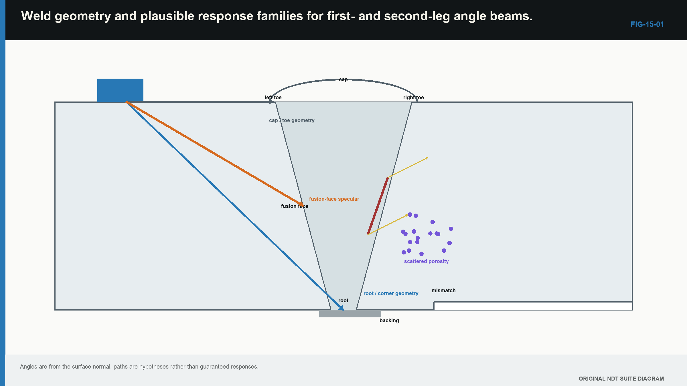
Notice that several different causes can occupy nearby screen times, so the drawing starts the test rather than ending it.
15.2 Translate the weld process into likely orientation
Discontinuity names become useful when linked to how they form. Lack of sidewall fusion commonly follows a preparation face. Inter-run lack of fusion follows a bead boundary and may curve. Incomplete penetration occupies the intended root-fusion region. Solidification cracking can follow the weld centreline. Heat-affected-zone cracking may be longitudinal or transverse according to stress and structure. Slag or oxide can follow inter-run flow, while pores may occur alone, in clusters or as elongated wormholes.
Orientation changes reflection. A smooth planar face tends to return most sound when the beam meets it near normal incidence. A rough or branched crack has many local face directions and can scatter more broadly. A tip or edge diffracts sound over many directions, usually at lower amplitude than a favourable face return. Rounded pores scatter, and a cluster can create a fluctuating group of echoes as the beam moves.
These are tendencies, not screen signatures. A slag line can behave like a plane, a crack face can be rough, and root geometry can give a sharp high echo. Use process knowledge to choose tests, never as the only reason for a label.
15.3 Make the first screen trustworthy
Confirm range, zero, angle or index, sensitivity, gate position and scan-surface transfer before interpreting. Keep the response below saturation. A clipped peak hides amplitude change and can make separate echoes appear as one broad signal. Check coupling with a suitable stable response while moving.
Plot the echo using the declared path and leg. Compare that position with the measured weld sketch, not merely with a coloured cursor labelled “root.” If it lies on expected geometry, geometry becomes a live explanation. If it lies on a plausible fusion face, a planar weld feature becomes plausible. Neither conclusion is final.
Repeatability also matters. Re-find the response after lifting and replacing the probe. A response that depends on one unstable contact position should first trigger a surface and coupling check.
15.4 Move the probe to create evidence
A static peak gives little information. Probe movement changes incidence, illuminated area and path. Use that change deliberately.
Forward and backward movement tests sound path and angle dependence. Lateral movement shows how the response changes across the beam. Orbital movement varies the approach around a plotted point. Skew rotates the beam plane and is essential for transverse or tilted features. Scanning from the other side changes which faces and tips are favourably illuminated.
Describe what happens before interpreting it. Record the position of maximum response, the movement over which the echo remains observable, whether it separates into peaks, and which direction strengthens or loses it. A fast rise and fall may come from a compact reflector or simply from a narrow field crossing an edge. A long response may be physical length, beam footprint, several reflectors or changing surface geometry.
15.5 Compare competing explanations
Use a short interpretation table rather than one favourite story. For each response, compare at least expected geometry, a planar weld-related feature and a distributed or volumetric feature.
| Observation | Expected geometry | Planar weld-related feature | Distributed or volumetric feature |
|---|---|---|---|
| Plotted position | Matches root, cap, backing or known surface | Lies on a plausible fusion or crack plane | Occupies weld volume without one clear plane |
| Directional behaviour | Repeats at paths predicted by the drawing | Often peaks strongly from a favourable direction | Often broader or irregular |
| Probe movement | Stays tied to a component boundary | Changes with incidence and may show face or tips | Fluctuates as parts of the group enter the beam |
| Other-side scan | Follows corrected geometry | May strengthen or weaken because the face orientation changes | May persist but with a different pattern |
| Independent check | Measured dimensions support it | Another angle or tip evidence supports a plane | Another method may support a distributed region |
Table 15.1
The table is not a scoring system. Its value is that it exposes which observation supports each physical model and which expected observation is missing.
| Worked example · Compare root and fusion-face explanations WE-15-01 Given: A response in a 25 mm V-butt weld plots 2 mm above the measured root and 3 mm onto a fusion face. It peaks with a 60 degree shear beam from side A, falls by 12 dB with a 45 degree beam and is barely visible from side B. Actual thickness and root position have been checked. Find: Which explanation better fits the stated evidence: symmetric root geometry or a planar fusion-face reflector. Steps: Compare position, directionality and opposite-side behaviour. Corrected root geometry should plot at the root and have a related path from the other side. A planar face can peak from the direction closest to normal incidence and weaken strongly from another direction. Answer: The planar fusion-face explanation fits more of the observations. What it means in practice: The result supports a planar characterisation. It does not prove the exact metallurgical type or determine acceptance. Common mistake: Treating the 12 dB change alone as a unique defect signature. |
|---|
15.6 Test known weld geometry
Roots, caps, toes, backing and counterbores can all return or redirect sound. Mismatch moves the root relative to the centreline and can make a response appear from only one side. A later-leg beam may also meet the same boundary at an unexpected position if the wrong thickness is used.
Where safe and accessible, compare the response with adjacent known geometry. Change the probe position and calculate how an echo from that boundary should move. A genuine geometry response should follow the component datum. A discontinuity close to the geometry may follow a related but distinct track.
A planar face meeting a surface can form a corner trap. Energy reflects between the two surfaces and returns efficiently. A weld root can create a similar path, so high amplitude is not proof of a surface-breaking crack. Location, predicted time and movement must agree.
| Worked example · Check a corner-trap path WE-15-03 Given: A vertical planar reflector meets the back wall at 25 mm depth. With a 45 degree shear beam, the probe index is positioned so that the horizontal and vertical offsets to the corner are both 25 mm. Shear velocity is 3,230 m/s. Find: The one-way path and predicted pulse-echo time. Steps: The one-way path is sqrt(25^2 + 25^2) = 35.36 mm. The round-trip path is 70.71 mm. Time is 70.71 mm / 3.230 mm per microsecond = 21.89 microseconds. Answer: The predicted pulse-echo time is about 21.9 microseconds. What it means in practice: Time agreement supports the corner-path explanation but cannot say whether the vertical face is cracking, a fusion boundary or known geometry. Common mistake: Calling a strong echo a crack without first modelling the efficient geometric return. |
|---|
15.7 Recognise a changed wave mode
A shear wave hitting a boundary can produce a longitudinal component, and a longitudinal wave can produce shear. Because the modes travel at different speeds, a mixed path will be misplaced if the display treats the entire journey as one mode. Wedge echoes and surface waves can add other repeatable signals.
State the candidate path in segments. The physical relationship is simple: total time equals the time spent in each segment added together. Each segment time is its length divided by the speed of its wave mode.
| (15.1) Travel time along a path containing more than one wave mode · EQ-15-01 Where: t_total = predicted total travel time (s); L_i = length of segment i (m); c_i = wave speed in segment i (m/s) Model limits: the candidate path and wave mode of every segment are declared; each segment can be treated as having a suitable constant speed; instrument and wedge delays have been corrected separately |
|---|
Use metres with metres per second, or millimetres with millimetres per microsecond. The units must match. The calculation tests whether a path could explain the time; it does not identify the reflector by itself.
| Worked example · Compare an all-shear and a mixed-mode path WE-15-02 Given: An echo arrives at 42.0 microseconds. Candidate A is a 136 mm all-shear return at 3.230 mm per microsecond. Candidate B contains 80 mm of shear path at 3.230 mm per microsecond and 35 mm of longitudinal path at 5.900 mm per microsecond. Find: Which candidate better matches the observed time. Steps: Candidate A gives 136 / 3.230 = 42.1 microseconds. Candidate B gives 80 / 3.230 + 35 / 5.900 = 24.77 + 5.93 = 30.70 microseconds. Answer: Candidate A, the all-shear path, matches the observed time much more closely. What it means in practice: The calculation makes the stated mixed path unlikely. Geometry and movement are still needed to identify the reflector. Common mistake: Choosing a path because its drawing looks plausible without checking its arrival time. |
|---|
15.8 Separate the face, the tips and the length seen on screen
A broad face echo and a tip echo answer different questions. Face amplitude depends strongly on orientation and illuminated area. A tip time can locate an extremity. A large face response can saturate or mask the smaller tip. Reducing gain or changing angle may separate them, but the changed setup needs a valid calibration identity.
The length over which an echo remains above a threshold is called response extent. It is not automatically discontinuity length. Beam footprint, threshold, directivity, encoder position and surface variation all affect the endpoints. A long planar feature can appear broken where its local direction reflects sound away. A short reflector can remain visible while the edge of a wide beam passes across it.
Report the observed response extent and the method used. Claim physical length only when the sizing method and its demonstrated performance support that claim.
15.9 Difficult welds need a different limit
Austenitic and dissimilar-metal welds can change velocity, attenuation and beam direction with grain orientation and polarisation. [R008] A nominal angle can skew, split or broaden. Structural response may hide weak tips. A response can plot neatly under an isotropic parent-metal model and still be wrongly located.
Warning signs include systematic location disagreement from opposite sides, strong direction-dependent loss, pulse broadening through the weld and known-reflector peaks displaced from prediction. Lower frequency, specialised probes, alternate modes, mapped fields or representative specimens may be required.
The Level 2 responsibility is not to invent a correction from an uncertain echo. It is to recognise when the approved simple model no longer explains the evidence, apply the permitted alternative checks and state the remaining limitation.
15.10 Characterise with restrained language
Evidence often supports one explanation more strongly without proving an exact discontinuity type. A report can say “planar response consistent with a fusion-face feature” and give its corrected position, observed extent and supporting directions. That is more useful than a confident but unsupported metallurgical label.
Independent observations strengthen the conclusion: corrected coordinate agreement, a new insonification direction, a distinct extremity response or another suitable method. Recolouring or filtering the same stored data may help viewing, but it does not create a new physical observation.
The conventional weld-response and interpretation foundation used here is consistent with the international UT training reference. [R001]
The final figure arranges the observations by the competing explanation they support or contradict.
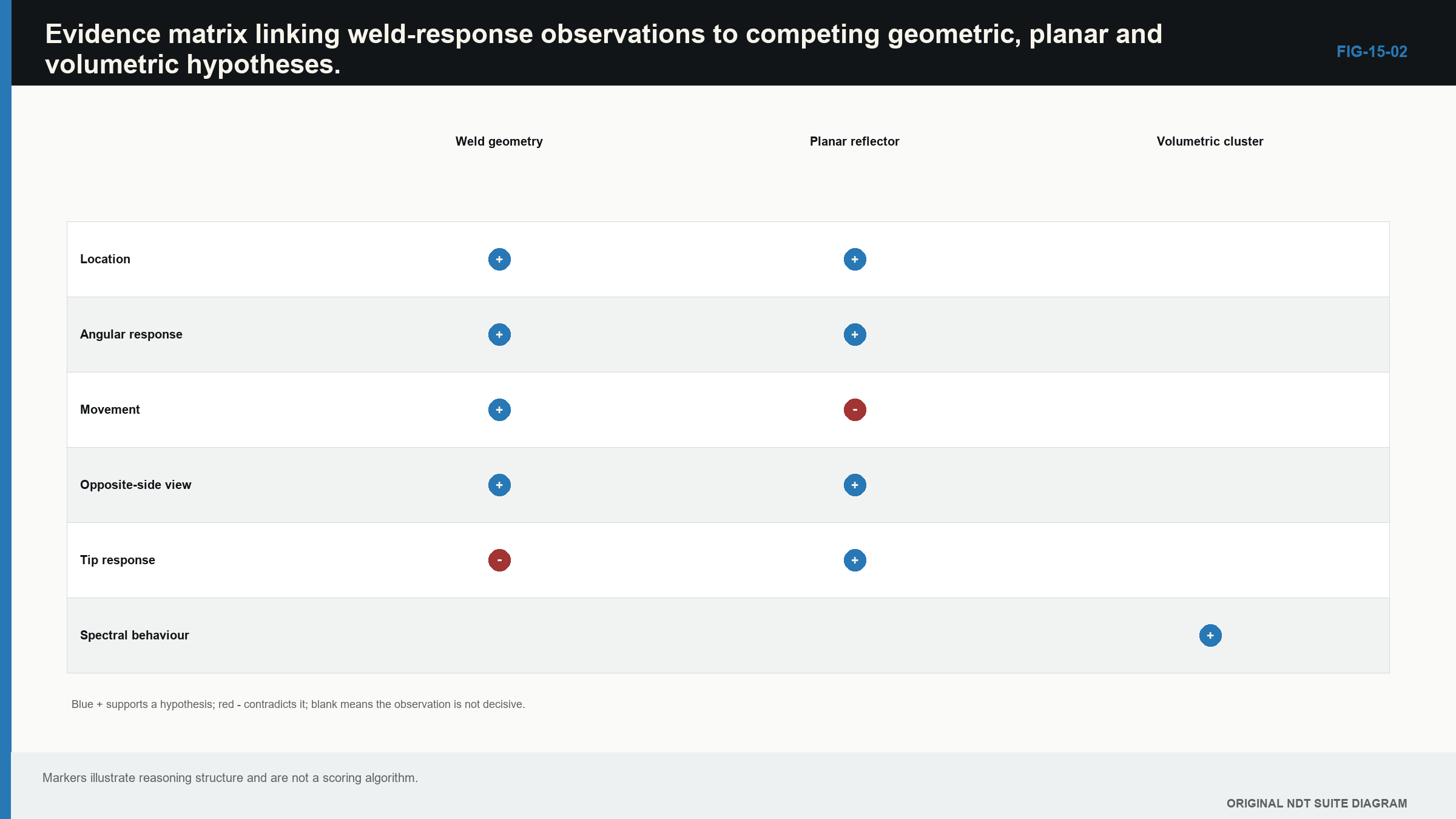
Notice that no single row produces a verdict; strength comes from several physically related observations.
In plain words
- Draw and measure the finished weld before trusting a plotted echo.
- Formation mechanism suggests likely orientation, not a guaranteed screen shape.
- Keep the signal unsaturated and the calibration valid before comparing responses.
- Probe movement and different directions turn one echo into a useful set of tests.
- Known weld geometry and mode-converted paths can imitate relevant discontinuities.
- Response extent is not automatically physical discontinuity length.
- Report the strongest supported characterisation and keep remaining alternatives visible.
Key terms
- Specular response: strong mirror-like return from a favourably oriented face.
- Tip diffraction: lower-amplitude sound spreading from an edge or extremity.
- Corner trap: efficient return involving two surfaces that meet.
- Mode-converted path: a path containing more than one wave mode.
- Response extent: the scan distance or region over which an echo meets a stated display rule.
Key relationships
- Planar-face response generally strengthens as incidence approaches the face normal.
- Total mixed-path time is the sum of segment length / segment wave speed.
- Observed response extent combines reflector, beam, scan path and threshold effects.
- Agreement of position, movement and a separate physical view is stronger than amplitude alone.
Common mix-ups
- Root-position echo does not automatically mean harmless root geometry.
- A high echo is not automatically a large discontinuity.
- A crack does not always give one sharp response, and porosity does not always give one broad response.
- Time agreement makes a path plausible; it does not prove the reflector type.
- A second display of the same data is not independent evidence.
Bridge to Chapter 16
This chapter has built the physical hypotheses. Chapter 16 turns them into a repeatable interpretation sequence: prove the data are valid, locate the response, test competing causes, decide what the evidence supports and report the result without hiding uncertainty.
Sources and further study
- [R001]
- [R008]
Study and revision only. This is not an approved inspection procedure, acceptance criterion or qualification.