
CHAPTER 37 · Phased Array Ultrasonics Level 3
From Ray Lines to the Real Array Field
In this chapter · 25 sections
Why this matters
A sector plot can show every centreline ray crossing a weld, yet a reference target near one edge of the sector remains weak and unstable. Nothing is necessarily wrong with the plot. It answered a geometry question, while the examination needs an energy-and-response answer. A PAUT Level 3 must know when a ray is enough, when a field calculation is needed and when only a measured complete-system response can support the claim. This chapter rebuilds the familiar ray as a wave-interference field and turns that model into practical choices about aperture, focus, steering, validation and reporting.
What you already need
- How PAUT elements, active apertures, focal laws and sector scans work at Level 2.
- The distinction between centreline, beam width, side lobes and grating lobes.
- Basic phase, wavelength, frequency and dB comparisons.
- The difference between detection, coverage, resolution and sizing.
- How a reference reflector and a service target can return sound differently.
What you will learn
- Explain why a ray path cannot describe sensitivity around that path.
- Build the physical picture from element wavelets to an interference field.
- Interpret the phased-aperture sum and state its assumptions.
- Select field metrics and normalisation that match a technique decision.
- Compare analytical, numerical and measured evidence without overclaiming.
- Define the uncertainty and reproducibility information needed for a field-supported release.
Words you will meet
- Superposition: addition of wave contributions at the same place and time.
- Huygens construction: picture in which points on a wavefront act like small secondary sources.
- Angular spectrum: description of a field as plane-wave directions and spatial frequencies.
- Apodisation: deliberate weighting of elements across an aperture.
- Pulse-echo field: combined transmit, target-scattering and receive response.
- Normalisation: choice of the reference used to scale a plotted response.
- Reciprocity: source-receiver interchange relationship under suitable linear conditions.
- Point-spread response: measured or modelled image of a compact target.
- Aberration: field distortion caused by an incorrect or varying propagation model.
- Evidence domain: the conditions and target population for which evidence supports a claim.
37.1 Start with the decision the ray cannot answer
A ray states a possible direction and travel path. It quickly shows whether a nominal beam can enter the component, reach a region or complete a skip. It can expose a wrong exit point, an inaccessible probe position or a fusion face that no selected angle meets. That makes the ray one of the most useful PAUT design tools.
The ray carries no amplitude distribution. It does not show the active aperture width, element directivity, frequency content, transmit-receive sensitivity, side structure or target scattering. When a decision depends on any of those properties, the ray is necessary but incomplete.
Use a three-part screen. First, establish whether the nominal path is geometrically possible; a ray may answer. Second, establish how useful response is distributed around that path; a field model or beam measurement is needed. Third, establish whether the complete setup can detect or size the required target population; representative performance evidence is needed. Model complexity follows the decision, not the seniority of the reviewer.
The figure below compares those three descriptions for one inspection region.
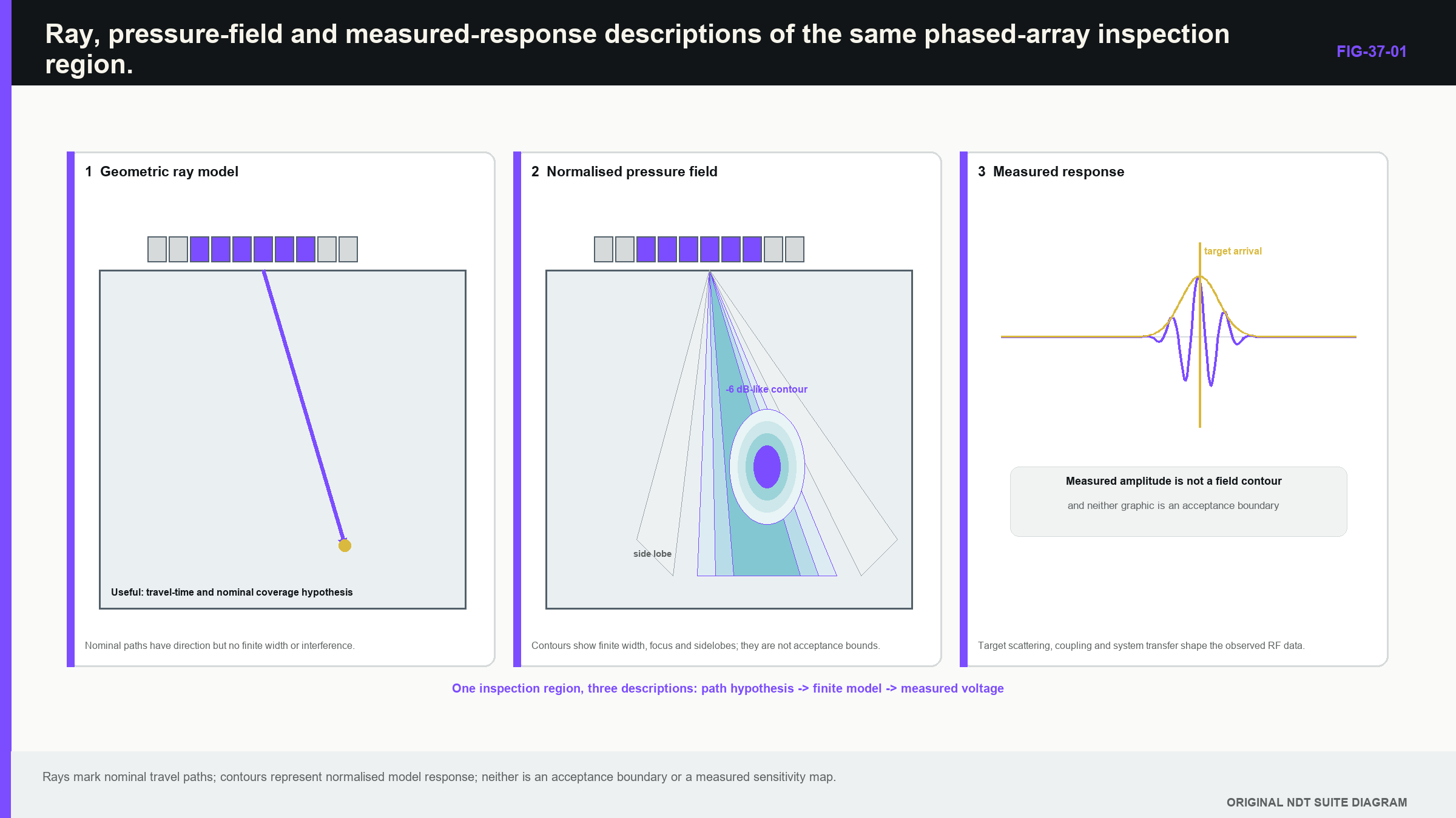
Notice that increasing model detail changes the supported question; it does not automatically make the answer more valid.
37.2 Reactivate the physical picture: many small wavelets
At Level 2, a focal law was introduced as controlled timing across several elements. The physical extension is that every loaded part of the aperture contributes a wavelet. At a point in the component, the wavelets arrive with different amplitudes and phases. Contributions that arrive in step reinforce one another; contributions that arrive out of step partly cancel.
The Huygens construction gives a useful picture. Treat each element face as a row of small secondary sources. A constant delay change from one element to the next tilts the combined wavefront and creates steering. A curved delay profile makes the wavelets meet near a selected point and creates focusing. The centreline is therefore not a rail carrying sound. It is a convenient direction associated with the combined field.
A real element is not a point source. Its finite width and elevation make response depend on angle. A wider element is normally more directional at the same wavelength, while a shorter wavelength also narrows the element pattern. A delay law can mathematically steer a main array maximum into a direction where each element radiates poorly. Field estimation must therefore combine the array interference pattern with element response.
Construction also matters. Matching layers, backing, electrode geometry, cabling, wedge loading and electrical impedance affect centre frequency, bandwidth, ring-down and sensitivity. Nominal frequency, pitch and element count do not prove that replacement probes produce the same pulse or field. Reference-block research supports treating probe construction and loading as measurement variables rather than catalogue trivia. [R010]
37.3 Read the aperture-sum model without needing a degree
The formal field model adds the element contributions. Each contribution has three practical parts: how strongly the element is weighted, how the element and acoustic path transfer energy to the point, and how much phase is created by propagation plus electronic delay.
| (37.1) Narrowband phased-aperture field sum · EQ-37-01 Where: p = complex pressure or displacement proxy at position r; r = field position (m); omega = angular frequency (rad/s); a_n = weighting of element n; h_n = element-and-path transfer term; T_n = propagation time from element n to r (s); tau_n = applied electronic delay (s); j = square root of -1 Model limits: linear propagation; one declared harmonic component; coherent excitation; element and path terms suitable for the stated mode, wedge, interfaces and plotted quantity |
|---|
The observable supported by this equation may be focal position, relative field magnitude, main-lobe width or side structure. It is not automatically a received A-scan or detection probability. Reflector scattering, receive response, pulse bandwidth, attenuation and processing may still need to be added.
At the intended focus, the delay law tries to make the phase terms align. Away from that point, the phases separate and the sum changes. Changing a_n is apodisation. Reducing edge weights commonly lowers side lobes while widening the main response and reducing coherent gain. Disabling elements changes both aperture extent and spatial sampling. The complete beam identity therefore includes active elements, weights, delays and frequency response, not only a law name.
Sensitivity case. Suppose one delay is changed by a small amount. The phase error grows with frequency, so high-frequency parts of the pulse lose coherence first. If one element is weak, its amplitude term changes. If the wedge velocity is wrong, many travel-time terms change in a structured pattern. This is why Level 3 review studies the pattern of error across the aperture rather than treating every input as an isolated tolerance.
37.4 Angular spectrum: the same field seen by direction
The angular-spectrum view starts from the aperture distribution and describes which plane-wave directions it contains. A wider finite aperture produces a narrower main angular distribution. Steering shifts the distribution. Apodisation reshapes it. Periodic element spacing samples it and produces repeated spatial spectra.
This view explains why grating lobes are spatial aliases. Two different directions can produce the same phase progression at the sampled element positions. If a repeated spectrum falls inside the range of propagating directions, energy can appear in an unwanted beam. Chapter 39 develops the design mathematics; here the important bridge is that grating lobes are not coloured display artefacts. They begin in how the physical aperture samples phase.
Huygens and angular-spectrum descriptions are not competing truths. Huygens wavelets make delay and interface construction intuitive. Angular spectra make aperture width, element pitch and side structure easier to reason about. Full numerical methods become useful when boundaries, curvature, anisotropy or multiple scattering break the simpler homogeneous model.
37.5 Near field, focus and bandwidth
The near field contains rapid interference variation. Changing active aperture or frequency changes that structure, and a focal law deliberately reshapes it. One conventional near-field length cannot describe every aperture and law in a PAUT sequence.
A stated focus needs a definition. It may mean the location of peak transmit pressure, peak pulse-echo response from a selected target or the centre of a chosen amplitude contour. The usable focal zone may be defined by a 6 dB limit, another amplitude rule or an application performance condition. Without the quantity, plane and threshold, a quoted focal depth is incomplete.
Increasing aperture generally narrows the main lobe in an ideal model. Steering reduces the projected aperture and may broaden the response. At large angles, element directivity and wedge-interface transmission can reduce sensitivity even when delays remain valid. A shallow nominated focus may also be limited by interface response, pulse duration and the short distance available for the field to form.
A pulse contains a frequency band. Each component has a different wavelength, phase error and lobe structure. The time-domain field is the combined result after transducer, wedge, material and receive weighting. A centre-frequency contour is useful for comparison, but it must not be presented as the only state of a broadband pulse.
Failure case: the sharp but fragile focus. A nominal model gives a narrow focus exactly on a weld-fusion face. A small credible velocity change moves the peak away and doubles side response near the root. The broader alternative law has lower nominal peak amplitude but keeps the whole target region within its validated contour. The Level 3 decision may favour the broader field because robust coverage matters more than the best nominal spot.
37.6 Pulse-echo response includes the target
Pulse-echo sensitivity contains a transmit journey and a receive journey. Under reciprocal linear conditions, a useful approximation combines transmit field and receive sensitivity at the target. Using the same aperture and focus both ways can make the two-way response narrower than the transmit-only field. Different receive apertures or dynamic receive laws can create asymmetry and depth dependence.
The target also matters. A small sphere, side-drilled hole, flat-bottom hole and planar crack do not sample the field in the same way. A compact target samples a local region. A broad planar target integrates phase over its face; parts of the return can even cancel. A smooth planar face can be weak when not favourably oriented despite lying inside a strong point-target contour.
A measured target scan is therefore a complete response involving field, target, motion increment, electronics and processing. Calling it a beam map is acceptable only when the target, contour convention and processing are retained. A cylindrical reference can test field continuity and timing, while a planar target challenges orientation and specular response. Neither proves every service target.
Reciprocity can challenge a linear model. Swapping source and receiver should preserve the transfer relationship under reciprocal conditions, although electronics and processing can break measured symmetry. A material difference after endpoint interchange can reveal a coordinate, boundary, polarisation or implementation error.
37.7 Choose metrics that answer the design decision
Beam width is not one universal number. A 6 dB target-response width, first-zero width and full width at half maximum use different boundaries. The result also depends on plane, depth, frequency, target and whether the field is transmit-only or pulse-echo.
Focal quality may be described by peak-position error, contour dimensions, side-lobe ratio, energy within a target zone, steering loss and robustness to plausible change. Use at least one metric for the desired response and one for unwanted response. A narrow main lobe without a side-structure or sensitivity measure can reward a field that is sharp but unusable.
Normalisation changes the visual conclusion. Scaling every law to its own maximum hides steering loss by construction. Scaling all laws to one common reference retains relative loss but can compress weak fields. Both can be useful when named. A uniform-sensitivity claim cannot rely only on per-law normalisation.
The same discipline applies to frequency-resolved fields. Report frequency range, spacing, source spectrum, attenuation model and any time-domain window. Truncation or an undocumented window can create ringing in a simulated pulse. Comparing peak magnitude alone can hide arrival-time and pulse-shape changes that affect gating and resolution.
37.8 Worked design calculation: footprint from a declared contour
For a simple far-field check, a measured or otherwise established contour half-angle can be projected to a target plane. In words, full width equals twice the distance multiplied by the tangent of the declared half-angle.
| (37.2) Approximate full width from a declared contour half-angle · EQ-37-02 Where: w = full width at the stated contour (m); z = distance from the effective aperture along the centreline (m); alpha = independently established contour half-angle (degrees or radians used consistently) Model limits: symmetric straight spreading in the stated plane; contour already established by a declared model or measurement; no claim of physical resolution or detection probability |
|---|
| Worked example · Turn a measured contour angle into a footprint WE-37-01 Given: A pulse-echo field map at a selected depth gives a symmetric 6 dB half-angle of 4.0 degrees. The target plane is 50 mm from the effective aperture along the centreline. Find: The approximate full 6 dB width at that plane. Steps: Use w = 2 z tan(alpha). Carry the distance in millimetres because the result is required in millimetres. w = 2 x 50 mm x tan(4.0 degrees) = 6.99 mm. Answer: The approximate full width is 7.0 mm under the stated contour and geometric model. Technical implication: The centreline ray cannot supply this width. The calculated footprint still depends on the measured contour, target response and plane, and it does not establish axial resolution, side-lobe level or target detectability. Common mistake: Reporting the 7.0 mm result as universal resolution or using a first-zero angle as though it were the measured 6 dB contour. |
|---|
A quick sense check is useful: at small angle, width should grow almost in proportion to distance. Doubling the plane distance would approximately double the result. If a calculation predicts narrowing with distance under this spreading model, the sign or geometry is wrong.
37.9 Design case: choose the evidence ladder
A Level 3 must decide how far to progress from simple model to measured proof. Consider a sector scan of a ferritic weld using a conventional linear array. Rays confirm access and show all required zones reached. A homogeneous field model then compares aperture sizes, maximum steering and focal depth. Measured compact-target scans verify focus position and side structure at shallow, middle and deep locations. Planar targets finally challenge orientation response.
This chain has different failure coverage. The ray finds impossible geometry. The model exposes aperture and parameter sensitivity. The compact-target scan includes probe construction and wedge loading. The planar target tests a service-relevant scattering mechanism. Agreement across these partly independent layers builds confidence; disagreement identifies the assumption requiring investigation.
The same chain may be inadequate in cast austenitic stainless steel. Measurements show that microstructure can distort fields and reduce coherence. [R012] Low-frequency arrays have improved penetration in particular thick-section applications, but that evidence remains tied to probe, aperture, scan spacing, material and specimens. [R011] In this case, representative-material mapping and target demonstrations carry more weight, and the supported evidence domain becomes narrower.
37.10 Failure and substitution case: the replacement probe
A replacement probe has the same printed frequency, pitch and element count. A common-reference scan restores peak amplitude with 2 dB additional gain, yet the off-axis response is broader and the high-angle laws lose more signal.
Gain can align one amplitude. It cannot restore a different angular spectrum, pulse bandwidth or field width. The field-supported claims affected may include angular coverage, response separation and sizing bias. Appropriate change evidence includes an element map, bandwidth or pulse comparison, target field scan and representative performance cases selected from the original qualification boundary.
If only peak amplitude is compared, the substitution can appear equivalent while the property driving coverage has changed. This is the evidence-boundary lesson: nominal identity plus one reference point is input evidence, not complete output equivalence. The array flexibility described in PAUT reviews depends on the realised aperture and field, not the label alone. [R016]
37.11 Three-dimensional and complex-path limits
A one-dimensional linear array is often modelled only in its active plane. The fixed elevation aperture still controls out-of-plane width. A skewed or finite-length reflector can lie outside the useful elevation field even when a two-dimensional sector covers its projected coordinate. Wedge roof angle, curvature and elevation focus can also shift the three-dimensional field.
Three-dimensional modelling becomes important for nozzles, curved welds, matrix arrays and targets that do not extend uniformly out of plane. If a two-dimensional model remains, its excluded dimension needs an elevation estimate or representative demonstration. The limitation belongs with the coverage claim, not in an appendix nobody reads until after a miss.
Anisotropy adds another limit. Phase-front direction and energy direction can differ, so a scalar isotropic contour may place the focus while useful energy follows another path. A model may still reproduce arrival time yet fail beam direction or amplitude. Chapter 43 develops a diagnostic hierarchy for these components.
37.12 Calibration, validation and uncertainty of a field result
Field-model calibration adjusts uncertain inputs, such as effective element size, source spectrum or attenuation, to selected measurements. Validation tests other measurements not used in that adjustment. Using the same map for both produces optimistic agreement.
Several parameter sets may match one centreline amplitude. Source strength, attenuation and target response can trade. Adding off-axis width, arrival time and pulse shape provides more independent constraints. If parameters cannot be identified, retain an uncertainty range or bounded empirical correction rather than one authoritative fitted curve.
A useful sensitivity study perturbs velocity, wedge position, element response, spectrum and target coordinate across credible ranges. Report changes in focus position, contour width, steering loss and side-lobe ratio. Measured maps also have uncertainty from target placement, mechanics, coupling and repeatability. Repeat with remounting and both scan directions to separate stable displacement from random texture.
Evidence-boundary case. A nominal model and one measured map agree within 0.3 mm at the central target, while repeat remounting varies by 0.4 mm. The data do not support a precise 0.3 mm model correction because the difference is smaller than the repeatability scale. The defensible outcome is agreement within the demonstrated measurement spread, plus a wider positional bound for the qualified region.
37.13 Minimum record and release test
A reproducible field record contains element geometry, aperture, weights, delays, source spectrum, wedge and material model, coordinate grid, plotted quantity, normalisation, software identity and reference evidence. It retains numeric field data where possible, not only a raster image. Every metric is linked to the inspection decision it supports.
The release test is practical. Another competent analyst must be able to reproduce the plotted quantity, and a measured target must challenge the region used in the claim. If either condition is absent, the field remains development evidence. The strongest package combines analytical scale checks, independently verified calculations and complete-system measurements because their errors are not identical. [R010] [R011] [R012] [R016]
37.14 Substitution case: the same footprint hides a different field
Two probe and wedge assemblies produce almost the same centreline footprint on a side-drilled hole. The replacement assembly is therefore proposed as equivalent. A full field comparison then shows that its main response is slightly broader, its high-angle energy is lower and one off-axis region is stronger.
The centreline footprint is one observable. It does not fully describe transmit-receive sensitivity, angular support or side structure. A change in element frequency response, elevation aperture, wedge attenuation or channel weighting can preserve the peak coordinate while changing the rest of the field.
Begin the change review with the qualified claims. If the technique relies only on broad detection of favourably oriented targets near the centreline, the observed difference may remain inside demonstrated margin. If it relies on weak tip response at the steering boundary, the lower high-angle field can affect sizing even though the reference hole looks normal.
Compare like quantities under one normalisation. Retain absolute or reference-linked amplitude where sensitivity matters, because normalising every map to its own peak would conceal the energy change. Compare contour position, width, side-response ratio and frequency-resolved behaviour at the field regions linked to the target population.
Next challenge the model with complete-system targets. A small reflector tests local field position. A planar target tests orientation support. A representative geometry feature tests whether the stronger off-axis region can create a false call. Repeat mounting so assembly-placement variation is not confused with a stable design difference.
The outcome can be output specific. Centreline location may remain comparable while high-angle detection and sizing require further evidence or a narrower range. This is why field release records contain quantities, normalisation and evidence domain rather than one attractive beam picture. [R010] [R011] [R012] [R016]
In plain words
- A ray proves a possible path, not useful sensitivity around that path.
- The array field is the sum of finite element responses with controlled timing and weighting.
- Huygens wavelets explain steering and focusing, while angular spectra explain aperture width and spatial aliasing.
- The complete pulse-echo response includes transmit field, reflector scattering and receive sensitivity.
- Beam width, focus and steering loss need declared quantities, planes, thresholds and normalisation.
- A sharp nominal focus can be inferior to a broader field that remains stable under credible variation.
- Model calibration and validation require different evidence.
- Field-supported release needs reproducible inputs, sensitivity results and measured complete-system challenges.
Formal synthesis
Array-field theory extends Level 2 ray and focal-law knowledge into a controlled measurement model. The narrowband aperture sum exposes element weights, transfer functions, travel times and electronic delays; broadband and pulse-echo predictions add spectrum, receive response and target scattering. A Level 3 selects the least complex model that can answer the design decision, verifies its implementation, validates its relevant observables and preserves the model's evidence domain.
Key terms
- Superposition: addition of the element contributions that form the field.
- Huygens construction: wavelet picture used to understand delayed wavefront formation.
- Angular spectrum: representation of aperture output by direction and spatial frequency.
- Apodisation: controlled change of element weights across the aperture.
- Pulse-echo field: combined transmit, scattering and receive response.
- Normalisation: declared reference used to scale field values or laws.
- Evidence domain: target, component and configuration range supported by the evidence.
Key relationships
- EQ-37-01 adds complex element contributions; phase alignment creates the desired field and phase error degrades it.
- EQ-37-02 projects an independently established contour angle into a geometric width, not a universal resolution value.
- Larger ideal aperture normally narrows main response, while apodisation trades side structure against width and coherent gain.
Common mix-ups
- Ray coverage is not demonstrated sensitivity coverage.
- A transmit-only pressure contour is not a complete pulse-echo target response.
- Per-law normalisation is not evidence of equal absolute sensitivity.
- A compact-target map is not automatically representative of a planar crack.
- Agreement after fitting is not independent validation.
Bridge to Chapter 38
This chapter showed what the aperture and its relative phases create. Chapter 38 works backward to the timing instructions: how element coordinates, wedge paths, component targets and coordinate transforms become a focal law, and how a Level 3 checks that the exported law still represents the intended physical path.
Sources and further study
- [R010]
- [R011]
- [R012]
- [R016]
Study and revision only. This is not an approved inspection procedure, acceptance criterion or qualification.