
CHAPTER 56 · FMC / TFM / PCI Level 3
TFM Mathematics and Imaging Functionals
In this chapter · 28 sections
Why this matters
TFM is often described as though it were one fixed image. It is more accurate to think of it as a family of calculations. Every calculation begins with the same practical act: predict when a response from one trial point should arrive in each A-scan, take the corresponding sample and combine the samples. The choices made during interpolation, weighting, summation, normalisation and display determine the numerical image.
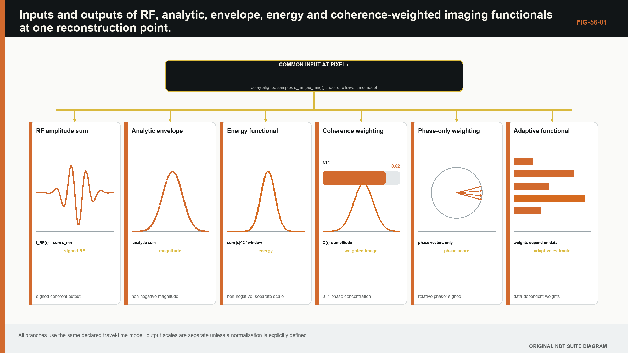
Start with one pixel and four traces. If the four selected waveform samples have the same sign and similar timing, their sum grows. If two are positive and two are negative, they can cancel. Taking an envelope before summing, summing complex analytic samples, or summing energy produces different values. The phrase imaging functional is simply the formal name for the complete calculation that maps the stored data to the value of that pixel.
What you already need
- FMC stores separate transmit-receive A-scans.
- A travel-time model predicts which sample belongs to a trial image point.
- RF samples have sign and phase, while an envelope is non-negative.
- Pixel spacing and the selected aperture can alter an image.
What you will learn
You will write and interpret a practical delay-and-sum calculation; distinguish RF, analytic, envelope and energy products; explain weighting and normalisation; connect a point-spread response to resolution and artefacts; and document an imaging functional so another person can reproduce it.
Words you will meet
An imaging functional is the declared calculation used to turn data and a propagation model into one pixel value. A weight changes the contribution of a trace. Normalisation places a result on a declared scale, often accounting for contributor count or reference response. A point-spread function is the image produced by a small reference reflector under the chosen method. A Green function is a formal description of how a source at one place produces a response at another; it is introduced as an extension after the practical delay-and-sum picture is secure.
The Level 3 step
Level 3 does not require the learner to accept a software label as the method definition. The calculation, preprocessing order, units and assumptions become controlled technique information. The later Green-function and continuous formulations generalise the same one-pixel idea; they do not replace it with unrelated mathematics.
56.1 From a propagation model to an imaging functional
An imaging functional maps acquired data and a model to a value at each trial point. The travel-time model predicts which sample from each transmit-receive trace is associated with scattering at that point. The functional defines how those samples are interpolated, weighted, combined and displayed.
The label TFM often refers to delay-and-sum focusing across a full matrix, but implementation choices matter. Raw RF, analytic signal, envelope, energy, sign or phase may be combined. Weights may compensate aperture, directivity or path. Normalisation may vary with contributing channel count. Two images can share a family name while carrying different numerical meaning.
The foundational FMC/TFM work records every transmit-receive pair and focuses synthetically at each image point. [R017] Later multi-view formulations extend the path model. [R018] The mathematics should therefore expose pair data, travel time, interpolation, weight and output domain instead of relying on the acronym.
56.2 A Green-function view
In a linear medium, a Green function describes response at a receiver from an impulsive source at another point under stated boundary conditions. A defect or material contrast scatters the incident field. In a Born-like single-scattering approximation, measured data can be expressed as an integral of transmit Green function, local scattering strength and receive Green function over the component.
Imaging backprojects the data with an approximate adjoint of that forward model. Delay-and-sum is a practical time-domain backprojection: for each candidate point, predict transmit and receive travel time and collect corresponding trace samples. It is not a full inverse solution because amplitude, multiple scattering and finite bandwidth are simplified.
This view clarifies model mismatch. If the Green function assumes a direct isotropic path but the component is layered or anisotropic, samples from a real target fail to align. The image can blur, shift or create artefacts. A stronger focusing functional cannot compensate for a wrong forward model indefinitely.
56.3 Continuous and discrete formulations
For a continuous aperture, an idealised image integrates data over transmit and receive coordinates. A real array replaces that integral with a sum. Time is sampled, so the predicted delay rarely lands exactly on a stored sample. Interpolation estimates the trace value at that time.
| (56.1) Weighted discrete delay-and-sum functional · EQ-56-01 Where: I(r) = image value at point r; x_ij = measured trace for transmitter i and receiver j; L = declared time-interpolation operator; T_i and T_j = transmit and receive travel times; w_ij = declared pair weight Model limits: valid path model, linear superposition, available trace support at each predicted time and a declared signal domain |
|---|
The sum can be real or complex. Summing RF samples preserves sign and phase but a target peak can occur on positive or negative phase. Summing analytic signals produces a complex value whose magnitude gives a phase-insensitive envelope after coherent combination. Taking each trace envelope before summation removes some phase cancellation and defines a different functional.
56.4 Amplitude, envelope and energy
An RF sum S = sum x_k is coherent in the sense that signed samples add. Its absolute value or envelope may be displayed. An analytic sum Z = sum z_k coherently combines complex samples; |Z| is a common amplitude image. Summing |z_k| is incoherent envelope addition. Summing |z_k|^2 forms an energy-like value.
These operations respond differently to noise and phase error. Coherent sums can grow proportional to channel count in amplitude for perfectly aligned contributions, while uncorrelated noise grows more slowly in expected magnitude. Incoherent sums avoid cancellation but also add noise and geometry energy. Normalising by channel count changes scale but not the underlying response.
Calling every output amplitude is ambiguous. A display in decibels should state its linear precursor and reference. 20 log10 is appropriate for an amplitude ratio; 10 log10 is used for a power or energy ratio. Applying the wrong convention changes reported differences by a factor of two.
56.5 Coherent and incoherent pair sums
Pairwise FMC data contain redundant and complementary phase. A target that matches the model aligns many pairs. A directional planar reflector may be supported by a subset. Summing all pairs equally can dilute response with channels that have little target sensitivity or high noise.
Weights can restrict aperture, apply element directivity, compensate geometric spreading or down-weight poor channels. Each weight introduces a model. A weight derived from the same data can adapt to target response but may also learn noise or suppress unexpected flaws.
Coherent compounding across views requires phase compatibility. Images reconstructed with different mode sequences may have unrelated phase references. Summing their magnitudes is not the same as summing their complex values. Multi-view fusion should preserve which quantities are commensurate.
56.6 Normalisation
Without normalisation, a pixel supported by more pairs can have a larger value. Near ROI edges or path-validity boundaries, contributing count may change. Dividing by number of pairs controls one geometric bias. Normalising by sum of absolute weights controls another. Neither compensates target directivity or material attenuation automatically.
Global maximum normalisation makes every image peak equal and destroys absolute comparison. Per-view normalisation can make weak artefact-dominated views look as strong as validated views. If qualitative display uses such normalisation, quantitative analysis should retain a stable scale.
Reference-target normalisation can support comparison when acquisition and path are reproduced. Its transfer to other target morphologies is limited. The reference and interpolation rules should be part of the reconstruction recipe.
56.7 Point-spread functions
The point-spread function is the image of an idealised point scatterer under the acquisition, model and functional. It describes main-lobe dimensions and side structure as a function of position. Because aperture support and path change across an ROI, the PSF is spatially variant.
A measured small reflector is only an approximation to a point. Its finite size and scattering pattern convolve with system response. Simulated PSFs allow controlled point targets but depend on model fidelity. Comparing both reveals different uncertainties.
Resolution claims should state criterion and location. Rayleigh-like separation, -6 dB width and two-target valley criteria are not interchangeable. Pixel spacing must be fine enough to sample the PSF but does not define it.
56.8 Frequency-domain and wavenumber functionals
Time-domain TFM evaluates delays directly and is flexible for geometry. Frequency-wavenumber algorithms can reconstruct regular array data efficiently by exploiting Fourier structure. Their speed and artefacts depend on sampling, interpolation, geometry and implementation. [R020]
Comparisons show that frequency-domain methods can be faster but sensitive to parameters and material noise. [R021] An algorithm name does not guarantee equivalence. Benchmarking should compare coordinate, amplitude, PSF, artefacts and computational conditions on common data.
Frequency-domain formulations also clarify aperture and propagation spectra. Evanescent or unsupported components cannot be recovered by ordinary far-field measurements. Regularisation and filtering choices influence resolution and noise.
56.9 Naming and reproducibility
A reproducible method declaration should include acquisition architecture, path, velocity model, ROI, pixel spacing, signal preprocessing, interpolation, functional, weights, normalisation, output transform and software version. "TFM at 0.2 mm" is not enough.
Common labels may be defined by standards or industry documents, but protected definitions are not reconstructed here. ISO's public FMC/TFM scope confirms a general-use framework and application boundaries without supplying universal acceptance levels. [R047]
Regression datasets should include known simple cases. A single impulse can test interpolation. A symmetric point target can test coordinate symmetry. A zero or noise input can expose offsets. Pair-count boundaries can test normalisation. These cases verify implementation before application validation.
| Worked example · Coherent gain and phase cancellation WE-56-01 Known: Four equal unit-amplitude analytic samples contribute to one pixel. Case A has phases 0, 0, 0 and 0 degrees. Case B has phases 0, 180, 0 and 180 degrees. Find: Compare complex sum magnitude and incoherent energy sum. Method: Case A complex sum is 4, so magnitude is 4. Case B complex sum is 1 - 1 + 1 - 1 = 0. In both cases, sum of individual squared magnitudes is 4. Result: Coherent amplitude distinguishes alignment completely; the simple incoherent energy sum does not. Engineering meaning: A functional selects which information matters. Phase cancellation can indicate model mismatch, but it can also arise from target scattering or polarity; energy addition is robust to phase yet less selective. |
|---|
56.90 Technical extension: deriving, comparing and testing functionals
56.90.1 Adjoint interpretation
For a linear forward operator A mapping a scattering field to data, the adjoint A* maps residual data back into image space. Delay-and-sum resembles an adjoint when its travel times and weights represent the forward paths. The adjoint is not the inverse: it produces a blurred image governed by A* A, whose columns are point-spread functions.
This distinction explains why a bright image does not recover true scattering strength automatically. Deconvolution or iterative inversion attempts to account for A* A, but requires regularisation and a more complete model. TFM remains a powerful backprojection whose limits can be described without downgrading its practical value.
56.90.2 Dimensional meaning and calibration
Raw digitiser counts, volts, analytic magnitude and normalised image values have different units. Weights based on directivity or spreading can introduce further scale. If a quantitative amplitude is reported, trace the units and calibration through every operation.
Many images are intentionally relative. That is acceptable when the reference is declared and transfer limits are respected. A relative scale should not be renamed reflectivity unless the forward and calibration model supports that interpretation.
56.90.3 Weight design
Weights can model transmit amplitude, receive sensitivity, path transmission, geometric spreading, attenuation and noise variance. Multiplying many uncertain corrections can amplify error. A theoretically unbiased weight may produce unstable images where its denominator is small.
Regularised or clipped weights trade bias for robustness. The clipping limit becomes an essential parameter. Compare weighted and unweighted results on target and non-target cases to show what the correction changes.
56.90.4 Aperture support and pair validity
Not every pair contributes a physical path to every pixel. A validity mask can exclude total internal reflection, out-of-bounds interfaces, missing time support or element directivity limits. The contributing count and angular span should be retained as companion maps.
Normalising by pair count can equalise scale while hiding a narrow angular support. A support-quality metric should therefore include distribution, not only number. Ten neighbouring pairs do not equal ten widely diverse views.
56.90.5 Noise propagation
If trace noise is independent with variance sigma_k^2, variance of a weighted linear sum is sum |w_k|^2 sigma_k^2. Correlated electrical or grain noise adds covariance terms. Coherent noise can grow like a target and defeat the usual square-root channel-count intuition.
Noise estimates should come from representative time and component regions. Estimating noise after image-dependent thresholding biases it low. A covariance model can inform whitening or adaptive weights, but errors in that model alter the functional.
56.90.6 Functional comparison matrix
Compare functionals using common raw data, paths, ROI and display scale. Record localisation, PSF, target contrast, geometry response, noise distribution and runtime. A method can improve contrast by suppressing a legitimate target class, so populations must include varied scattering.
The comparison should separate algorithm development from confirmation. Selecting the best exponent or filter on the final specimen gives an optimistic result. Parameter robustness is part of performance.
56.90.7 Multi-view mathematical compatibility
Complex sums from different paths are not automatically phase compatible. Each path can have boundary phase shifts, polarisation and reference delays. Coherent cross-view summation requires a model for those phases. Magnitude fusion avoids phase reference but defines a nonlinear output.
A useful alternative is to retain a vector of view responses at each point and interpret it with a validated decision rule. This preserves path identity and supports uncertainty rather than collapsing everything into one number.
56.90.8 PSF as a matrix diagnostic
Computing PSFs across the ROI reveals spatial variation in width, orientation and side lobes. The Gram matrix of model columns reveals similarity between candidate scatterer locations. High off-diagonal similarity indicates that two locations or paths are hard to distinguish.
This provides a quantitative identifiability screen. It still reflects the assumed point-scatterer model and noise weighting, so extended reflectors need additional tests.
56.90.9 Numerical and model uncertainty
Interpolation, grid and precision create numerical variation. Velocity, geometry and scattering create model variation. They should be evaluated separately before combination because remedies differ. Refining a grid cannot fix velocity bias; calibrating velocity cannot fix an indexing bug.
Ensemble reconstruction can propagate uncertain inputs into distributions of peak coordinate, amplitude and morphology. If the peak jumps between lobes, reporting a mean coordinate is misleading; the multimodal outcome should remain visible.
56.90.10 Functional verification cases
Verification cases should include equal aligned impulses, alternating polarity, one missing pair, unequal weights, noise-only data and pixels with partial support. Expected values can be calculated by hand. A point-target simulation then tests the full travel-time and interpolation chain.
Regression should compare the linear precursor before display transformations. Log compression and colour maps can conceal small but important changes. [R017] [R018] [R020] [R021] [R047]
56.91 From backprojection to quantitative comparison
Quantitative comparison across images requires stable gain and functional scale. Reconstruct a reference target at several positions and paths without per-image maximum normalisation. Track pair support, weight sum and predicted transmission. Residual position dependence reveals incomplete correction or spatially varying PSF.
If an image is intended for sizing rather than amplitude evaluation, coordinate and boundary stability may be more important than absolute scale. Define the metric accordingly. An optimisation that equalises peak amplitude can distort PSF and threshold width.
Model-based amplitude corrections should be stress tested. Directivity or transmission coefficients approach small values at some angles; dividing by them creates large weights and noise. Regularisation limits should be justified through target and artefact performance.
For extended reflectors, the point-scatterer adjoint can map different parts into lobes or edges. Simulate or measure planar targets across orientation. A functional tuned to point targets may report fragmented planar morphology even with correct travel time.
Functional uncertainty can be assessed by reconstructing a controlled ensemble across velocity, geometry, interpolation, weight and noise. Separate coordinate variation, amplitude variation and topology changes. A topology change, such as one peak splitting into two, is not summarised well by pixelwise standard deviation.
Release documentation should include a symbolic equation and an executable reference case. The equation defines intent; the case detects implementation drift. Both are needed because prose names alone cannot distinguish envelope-before-sum from envelope-after-sum or alternative normalisations. [R017] [R018] [R020] [R021]
56.92 Functional sensitivity to scattering and preprocessing
Test a functional with point, planar, edge, rough and multiple reflectors. Record which channel phases and amplitudes each target produces. A functional that excels on point scatterers can fragment a plane; an envelope sum can retain a diffuse response that a coherent RF sum cancels.
Preprocessing sensitivity should include bandwidth, DC removal, time-zero correction and trace normalisation. Apply one change at a time and compare raw pair contributions at selected pixels. This reveals whether an image improvement comes from better model alignment, noise suppression or altered target weighting.
Weights and normalisation should be inspected as maps. A bright feature at a location where weight sum or pair support changes abruptly may be algorithmic. Retain unweighted and support-count companions during validation.
For quantitative use, propagate reference-target and reconstruction uncertainty into the image metric. If per-view scale is arbitrary, keep the output qualitative and avoid amplitude-style decibel evaluation. A stable qualitative domain is more defensible than an invented physical unit.
Finally, compare the optimised implementation with a transparent reference functional on small datasets. Differences should be explained by declared weights, interpolation or precision. An unexplained improvement is a defect candidate, not free resolution. [R017] [R018] [R020] [R021] [R047]
56.93 Functional release question
A functional is release ready when its equation, input domain, weights, normalisation and edge behaviour are fixed; hand-calculable cases pass; and target plus artefact populations support its intended outputs. A cleaner image alone is neither verification nor validation. [R017] [R021]
56.94 Functional scale check
Reconstruct a dataset after duplicating every valid pair. An unnormalised coherent sum should change predictably; a pair-count-normalised result should remain stable. Similar invariance tests expose hidden scaling and support-dependent behaviour before images are compared quantitatively. [R017]
56.95 Engineering check: preserve phase and units through the imaging chain
A TFM implementation can produce a plausible image while using inconsistent phase conventions. The verification set should include analytical signals with known delay, polarity and phase; symmetric transmitter-receiver pairs; and a point target at a known coordinate. The expected result is checked before envelope detection, because the envelope can conceal sign reversals and some phase errors. Time origin, interpolation convention, sample units and any analytic-signal transform belong in the algorithm record.
Amplitude also requires a declared convention. Summing raw voltage, normalised channel data or propagation-corrected contributions produces different image quantities. Comparing two reconstruction variants is meaningful only when their scaling and preprocessing are common or explicitly reconciled. A reference implementation should retain intermediate travel times and channel contributions for selected pixels, allowing disagreement to be traced to geometry, interpolation, weighting or summation instead of being diagnosed from the final colour map alone. [R011] [R016] [R023] [R024]
Chapter synthesis
TFM is an imaging-functional family built from acquisition data, travel-time models, interpolation, weights and a signal domain. A Green-function view links delay-and-sum to an approximate adjoint of the forward problem. RF, analytic, envelope and energy sums are different quantities. Normalisation controls support and scale but can hide weak views. PSFs describe spatially varying image response, not pixel size. Frequency-domain algorithms trade structure and speed against sampling assumptions. Reproducibility requires the complete reconstruction recipe rather than an acronym.
Key equations and relationships
| (56.2) Normalised weighted analytic image · EQ-56-02 Where: I_N = normalised image amplitude; z_k = analytic trace sample; T_k = predicted pair travel time; w_k = pair weight Model limits: denominator is nonzero and the chosen normalisation is appropriate to the comparison being made |
|---|
In plain words
- The chapter's central control is imaging functional, and its meaning must be stated before its mathematics or software implementation.
- A faster, sharper or cleaner result is not automatically a more reliable result.
- Every claimed improvement depends on a declared dataset, model, configuration and target population.
- Known reference cases and deliberately difficult cases reveal different weaknesses.
- Stored raw evidence, metadata and software identity make later review possible.
- The technical conclusion must remain inside the boundary demonstrated by the evidence.
Key terms in this chapter
The words introduced at the chapter opening are the minimum vocabulary for its Level 3 work. Use them consistently in the technique, validation record and report. Where a supplier uses a different label, record the supplier term without allowing it to replace the physical definition.
Common mix-ups
- Do not confuse a similar displayed image with equivalent retained information.
- Do not confuse software verification with physical validation of an inspection technique.
- Do not confuse an assumed model output with a directly observed quantity.
- Do not confuse a demonstrated result for one target population with universal capability.
Independent review checkpoint
Give a second competent reviewer the raw or reference data, the declared imaging functional method, the controlled configuration and the expected comparison outputs. The reviewer should be able to reproduce the important result without using an undocumented display adjustment or private software setting. Record the version, input identity, contributor or channel mask, model inputs, numerical tolerances and any excluded cases. Also record one observation that would contradict the preferred explanation. Where the result supports a decision, the reviewer records the nearest failure boundary and one realistic change that would trigger revalidation. This checkpoint does not turn independent review into a ceremonial signature. It tests whether the evidence chain is understandable, repeatable and honest about its limits.
Bridge forward
Chapter 57 examines the travel-time model that tells the functional which samples belong to each trial point.
Sources and further study
- [R011]
- [R016]
- [R017]
- [R018]
- [R020]
- [R021]
- [R023]
- [R024]
- [R047]
Study and revision only. This is not an approved inspection procedure, acceptance criterion or qualification.