From Phased Array Ultrasonic Testing to Record-First Matrix Imaging

Why this matters

A phased array ultrasonic testing setup can form useful beams while the component is being scanned. Matrix imaging changes where some of that work occurs. Full matrix capture records many separate element-to-element waveforms first. Total focusing then uses those stored waveforms to calculate an image. Phase coherence imaging can process the same timing evidence in another way; a learner who keeps acquisition, reconstruction, display and interpretation separate can compare the methods sensibly. A learner who blends them together can obtain a very sharp picture of the wrong assumption.

What you already need

• The conventional ultrasonic testing picture of a pulse leaving a probe and returning as an echo.
• The phased array ultrasonic testing ideas of elements, an active aperture and a focal law.
• Basic A-scan timing, gain, coupling, sound path and encoded-position knowledge.
• The difference between detecting, locating, characterising, sizing and evaluating a response.
• Confidence multiplying two whole-number counts.

What you will learn

• Explain what remains unchanged when moving from phased array testing to matrix imaging.
• Distinguish full matrix capture acquisition from total focusing reconstruction.
• Describe one matrix cell and one reconstructed pixel in plain language.
• Explain what phase coherence imaging emphasises without treating it as a defect detector with special powers.
• Separate acquisition, reconstruction, display and interpretation decisions.
• Decide which later changes can use stored data and which require new acquisition.

Words you will meet

• Full matrix capture: an acquisition that stores a declared set of transmitter-receiver A-scans separately.
• Total focusing method: an image calculation that aligns stored pair signals for each selected pixel.
• Matrix: a grid whose row identifies a transmitter and whose column identifies a receiver.
• Reconstruction: the calculation that turns stored waveform data and an acoustic model into an image.
• Pixel: one calculated location in a reconstruction region.
• Phase coherence imaging: processing that emphasises agreement in waveform phase or sign under a declared implementation.
• Evidence domain: the kind of quantity a display actually represents, such as amplitude or phase agreement.

46.1 Begin with the phased array picture you already know

In phased array ultrasonic testing (PAUT), several array elements can fire with controlled delays; the delayed wavelets reinforce along a chosen direction or around a chosen focus. The instrument repeats that process for a set of focal laws. A sectorial group might therefore contain a sequence of angles, while a linear group moves an active aperture along the array. The focal-law decisions are made before or during acquisition, and the stored beam A-scan normally contains signals already combined according to that law.

Nothing about the material changes when the acquisition name changes. Sound still travels through the wedge and component. Interfaces still reflect, transmit and convert modes. Reflector orientation still governs whether energy returns to the aperture. Frequency and bandwidth still affect penetration and separation. Coupling, surface condition, attenuation, geometry and noise can still limit the result; the array also remains a physical array with the same element positions, pitch, bandwidth and directivity.

The change is mainly informational. PAUT commonly stores a selected set of already beamformed conversations. Matrix acquisition can retain many elementary conversations separately. That extra record allows some focusing and path choices to be made later, but only inside what was actually captured.

46.2 One element, one conversation, then many

Start with one ordinary pitch-catch event. Element 6 transmits a short pulse. Element 19 listens and stores an A-scan; that A-scan is one conversation between a known transmitter and a known receiver. It contains signed waveform value against time, together with the effects of both element paths, the wedge, coupling, component and electronics.

Now let element 7 transmit while element 19 listens; the second trace describes a different pair geometry. Continue across the selected transmitters and receivers. Arrange the results as a grid; each row belongs to one transmitter, each column belongs to one receiver, and each cell contains one A-scan. That grid of separately identified conversations is the foundation of full matrix capture (FMC).

The word full must be tied to the declared element set; a conventional square FMC sequence commonly lets each selected element transmit in turn and records every selected receiver. Other systems can store a half matrix, a sparse selection, plane-wave data or another architecture; those approaches may be useful, but the acquisition record must be named honestly. A screen labelled TFM does not prove that full pulse-echo FMC exists behind it.

The following figure shows the crossover in the order the learner encounters it. Notice that the pair A-scans exist before any total-focusing pixel is calculated.

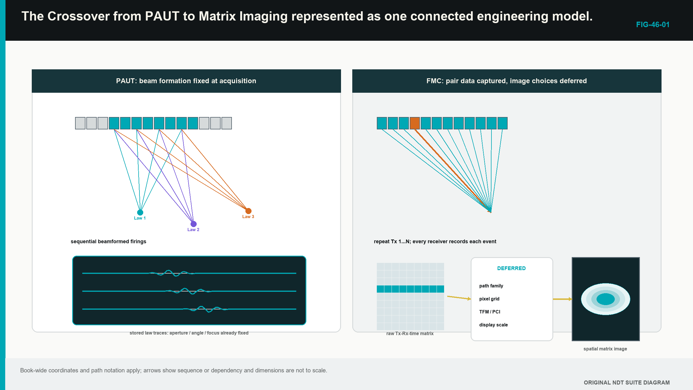
The useful observation is simple. PAUT chooses a limited set of beam combinations early. FMC preserves a larger set of elementary pair records. Neither approach is automatically superior; the right choice follows the inspection objective, demonstrated performance, scan speed, storage and review burden.

46.3 Count what FMC stores

If every selected transmitter is paired with every selected receiver, the number of stored A-scans is the transmit count multiplied by the receive count. The physical situation comes first: each firing produces one row of separately recorded receiver traces. The relationship is:

The count says how many pair records are expected; it does not prove that the traces are complete, correctly labelled, unclipped or useful. It also does not authorise removal of reciprocal pairs. Chapter 47 explains why the two directions can be compared and why comparison is not the same as automatic equality.

46.4 TFM uses the stored conversations later

The total focusing method (TFM) is a reconstruction family, not an acquisition event. Select one candidate image location. For every usable transmitter-receiver pair, the processor predicts how long sound would take to travel from the transmitter to that location and then to the receiver by the selected acoustic path. It selects the corresponding part of each A-scan, applies any declared weighting and combines the values; the calculation is repeated across the reconstruction region.

This gives a practical definition of one pixel. A pixel is the result of asking whether many stored pair traces contain mutually aligned evidence for one modelled location. It is not a little piece of the component photographed by the probe. Chapter 49 builds two pixels by hand and then introduces the delay-and-sum relationship.

The phrase focused everywhere is convenient but incomplete. TFM only calculates pixels inside the selected region of interest; it only uses the declared path, velocity, geometry, aperture and pair set. Acoustic resolution still depends on wavelength, bandwidth, effective aperture, depth, material and reflector behaviour. A grid with tiny squares cannot create energy outside the acquired field or restore information that never reached the receiver.

An incorrect model can still align some data; a wrong velocity may shift or blur the feature. A wrong component surface may cause the processor to sample the wrong times; an implausible mode or reflection may place real geometry energy at a false coordinate. TFM increases the available ways to inspect stored evidence; it does not suspend ordinary ultrasonic physics.

46.5 PCI changes the evidence being emphasised

An amplitude TFM image combines signed waveform values and normally displays a magnitude or envelope derived from that sum. Phase coherence imaging (PCI), in the amplitude-free implementation treated in this Level 2 part, emphasises how consistently the selected waveforms agree in phase or sign after their predicted delays. Amplitude is not the final pixel quantity in that route.

In plain words, several repeating waves can be compared by where each one sits in its cycle. When their cycle positions agree after the correct travel-time adjustment, the coherence response can be high. Diffracting crack tips and compact scatterers can become conspicuous because they may supply consistent timing across many pairs. Broad planar or interface responses can behave differently because only part of the aperture may receive favourable specular energy.

Agreement does not identify cause. Cross-talk, wedge ringing and component geometry can also repeat coherently. Very weak waveforms can give unstable phase because noise controls the apparent cycle position; a bright PCI feature is therefore phase-domain evidence under one model and implementation. It is not echo height in decibels, percentage full-screen height or a ready-made acceptance decision.

Some coherence methods multiply an amplitude image by a coherence factor instead of discarding amplitude. Their output differs from amplitude-free PCI. The acquisition type, processing family, software version and display scale must accompany the result. Chapters 47 and 52 build the necessary phase picture slowly before any formal coherence expression appears.

46.6 Keep four stages separate

Every advanced image can be traced through four stages. The first stage is acquisition. It includes probe and wedge identity, transmit sequence, receiver selection, gain, filters, sampling, time range, coupling, scan position and the signal form stored. A clipped trace or an omitted time window is already damaged at this stage.

The second stage is reconstruction. It includes velocities, component and wedge geometry, path family, aperture, pair selection, region of interest, grid, interpolation, weighting and algorithm. These decisions determine which stored samples contribute to each pixel.

The third stage is display. It includes envelope or phase treatment, normalisation, threshold, colour range, smoothing and screen resampling. Display choices can change prominence and appearance without changing the stored acoustic observations.

The fourth stage is interpretation. It includes path plausibility, component coordinates, known geometry, complementary views, characterisation, sizing, uncertainty and evaluation against the authorised source. Open technical material separates matrix acquisition from reconstruction and describes amplitude and phase-coherence evidence as different processing domains. Training references also place these methods inside a broader ultrasonic progression rather than granting automatic authority through a software label. [R017] [R025] [R046] [R047] [R060]

This separation makes troubleshooting practical. Poor coupling belongs first to acquisition. A misplaced known target can arise from acquisition timing or reconstruction geometry. An independently normalised image belongs to display. Calling a bright root response a crack belongs to interpretation. Changing a palette cannot repair a lost matrix, and changing velocity cannot repair clipping.

46.7 Trace a conclusion back to physical evidence

Three evidence layers sit inside the four-stage workflow. The first is the real acoustic interaction in the component, such as reflection, diffraction, scattering or mode conversion. The second is the sampled waveform affected by the probe, coupling, electronics and acquisition settings. The third is the image calculated from many waveform values.

A sound conclusion can move backward through those layers. A reported coordinate has a declared path. The path predicts arrival times. Representative transmitter-receiver traces contain support near those times. The support occurs across a useful aperture rather than one unexplained channel. A complementary view or known geometry then helps test the interpretation.

Production review does not require manual opening of every trace. The technique should, however, preserve access to the underlying evidence when a response is unexpected, contradictory or important. If only a screenshot remains, the reviewer cannot test a different justified region, inspect channel clipping or reproduce the processing route. The prettiest pixel in the folder then becomes an orphan with excellent colour grading.

46.8 What carries over from PAUT

The familiar controls remain valuable. Probe, wedge and element identity still matter. Wedge delay, material velocity and the component coordinate origin still control location. Encoder scale, direction and scan extent still connect data to the component. Channel health, coupling and saturation still determine whether the source waveforms are usable. Reference targets still help confirm location, coverage and response behaviour.

What needs fresh evidence is the part changed by the new information route. PAUT law verification does not by itself prove TFM coverage across a large region. A sensitivity curve used for amplitude data does not calibrate amplitude-free PCI. A stored PAUT beam does not become full matrix data because later software draws a TFM-style screen. A reconstruction path must be physically described and demonstrated for the region in which it will be used.

Element pitch, kerf, element width and aperture retain their physical meanings. Each element also has finite directivity, so a mathematically included pair may contribute little useful energy at an extreme angle. A larger pair count is not the same as a larger useful aperture. Detailed lobe, dynamic receive-focusing and spatial-sampling analysis remains in Parts V and VII, where it can be treated without burying this crossover picture.

46.9 A completed comparison case

A weld examination already has a PAUT sectorial technique. The technical team is considering FMC and TFM because the approved PAUT view gives limited tip evidence near one fusion face. The same array and wedge are placed over a representative specimen. The PAUT acquisition stores its declared focal-law responses. The FMC acquisition stores the pair traces over a time range long enough for the proposed direct and reflected paths.

The comparison begins with the task, not image sharpness. The PAUT baseline supplies known coverage, calibration behaviour, scan speed and existing evidence. The matrix route is checked for pair completeness, source signal range, position integrity and file size. One justified TFM view is then reconstructed. Its target positions and point-response shapes are compared with the specimen truth. Representative pair A-scans are inspected to show where the pixel support comes from.

Several later changes are now possible without another scan. A slightly expanded reconstruction region can be calculated because the required times were retained. A second physically justified path can be tested. Fixed-scale amplitude and phase-coherence views can be compared from the same source data. A higher pulser voltage, a missing off-diagonal time range, a changed array position or better coupling cannot be created afterwards; those changes require reacquisition.

The result is not a declaration that FMC/TFM replaces PAUT. It is a bounded comparison showing what the matrix method adds, what it costs and what remains unsupported. Scan time, storage, review load, false responses and difficult targets belong in the comparison beside the best-looking reflector.

46.10 Scope and authority at Level 2

This part develops the ability to follow, check and explain a defined FMC, TFM or PCI technique. It does not authorise a Level 2 technician to invent acceptance criteria, approve a new path, change an essential variable outside the permitted range or declare an unqualified method fit for production.

Work stops for technical direction when the component is outside the demonstrated material or geometry range, the required path cannot be drawn, source data are clipped or incomplete, verification fails, sizing is outside its demonstrated method, or the governing acceptance source is absent. A disagreement between amplitude and coherence views is also a reason to investigate, not an invitation to select whichever image is more dramatic.

Some decisions can be postponed from acquisition into reconstruction. Responsibility is not postponed with them. The acquisition still needs adequate time, bandwidth, pair coverage, position sampling and metadata. The reconstruction still needs a valid acoustic model. The interpretation still needs restraint and authority.

Step up

Part VII develops reduced acquisition, architecture equivalence, formal reconstruction functionals, path solvers, coherence families and validation at Level 3. Chapters 55 to 59 are the next route when the learner must design or defend those choices. Chapters 68, 69, 72 and 80 provide the engineering treatment of array sampling, signal processing, imaging algorithms and data-system capacity.

In plain words

• PAUT normally applies selected focusing decisions while the data are acquired.
• FMC records separately identified transmitter-receiver A-scans before TFM is calculated.
• TFM uses a path model to select and combine samples for each pixel.
• PCI emphasises phase or sign agreement and does not create an amplitude measurement.
• Acquisition, reconstruction, display and interpretation are different stages with different failure modes.
• Stored pair data allow some justified reprocessing, but they cannot restore information that was never captured.
• Matrix imaging extends ordinary ultrasonic physics; it does not replace it.
• Production use remains inside the approved technique and assigned authority.

Key terms

• FMC: separately retained A-scans for a declared transmitter-receiver pair set.
• TFM: pixel-by-pixel focusing performed from stored pair data and a declared path model.
• PCI: phase- or sign-agreement processing whose output scale belongs to the documented implementation.
• Matrix cell: one transmitter-receiver A-scan.
• Reconstruction: calculation that maps stored signals to selected image coordinates.
• Pixel: one calculated image location, not a physical photograph sample.
• Evidence domain: the quantity represented by an output, such as amplitude or coherence.

Key relationships

• N_trace = N_tx N_rx: the full ordered trace count equals transmitter count times receivers recorded per firing.
• PAUT law -> beamformed acquisition: selected delay combinations are commonly committed during acquisition.
• FMC traces + path model -> TFM pixels: stored pair data are sampled and combined during reconstruction.
• source waveform phase -> PCI: phase-domain output still depends on usable, unclipped source signals.

Common mix-ups

• FMC is an acquisition record; TFM is a reconstruction family.
• A TFM-labelled display does not prove that full FMC was stored.
• Fine pixels do not equal fine acoustic resolution.
• High coherence does not identify a reflector as a crack.
• A PAUT amplitude correction does not automatically apply to amplitude-free PCI.

Bridge to Chapter 47

Chapter 46 followed the whole crossover from PAUT to stored pair data and calculated images. Chapter 47 opens the matrix itself. It shows how rows, columns and cells organise A-scans, then introduces phase only after that grid is familiar.

Sources and further study

• [R017]
• [R025]
• [R046]
• [R047]
• [R060]