
CHAPTER 4 · Ultrasonics Level 1
What Sound Does at a Boundary
In this chapter · 18 sections
Why this matters
Every ultrasonic inspection contains boundaries. Sound crosses from probe to couplant, from couplant or wedge into the component, and from the component toward back walls, weld faces, coatings or discontinuities. At each boundary, some energy may return, some may continue and some may change direction or wave mode. A first-time learner does not need the full mathematics of elastic interfaces, but does need a correct picture of reflection, refraction, mode conversion and critical angles.
What you already need
- A pulse carries mechanical energy through a material.
- Longitudinal and shear waves use different particle motion and speeds.
- Wavelength and pulse length affect how separately echoes can be seen.
- Angles in this book are measured from the surface normal unless stated otherwise.
What you will learn
- Explain why an impedance change creates reflection.
- Calculate a simple normal-incidence reflection coefficient.
- Describe refraction and mode conversion at an angled boundary.
- Calculate simple refracted and critical angles.
- Explain why couplant thickness, roughness, curvature and layers change response.
- Use interface equations as estimates with visible assumptions.
Words you will meet
- Interface: boundary between two media or material regions.
- Impedance: a simple measure combining density and wave speed.
- Reflection: sound returned from a boundary.
- Refraction: change of wave direction when speed changes across a boundary.
- Mode conversion: creation of a different wave mode at a boundary.
4.1 A boundary divides the incoming sound
Press a dry probe onto steel and the A-scan may be poor or unstable. Add couplant and the response improves. The steel did not change. The path between probe and steel changed.
An interface can be the boundary between two separate materials, such as water and steel. It can also be a back wall, bond line, grain boundary, coating, crack face or gradual material transition. When a wave reaches an interface, the materials on the two sides must move and carry force in a compatible way. The incoming field is divided among reflected and transmitted fields.
A useful first comparison is specific acoustic impedance. For one stated wave mode, it combines material density with sound speed. In words:
acoustic impedance = density × wave speed
| (4.1) Specific acoustic impedance · EQ-04-01 Where: Z = specific acoustic impedance for the stated mode (Pa s/m); rho = density (kg/m^3); c = wave speed (m/s) Model limits: plane-wave relationship in a homogeneous medium |
|---|
When two media have equal impedance in the ideal one-dimensional model, no pressure wave is reflected at normal incidence. As the mismatch increases, reflection grows. Speed alone does not set the reflection because density is also part of impedance.
Air has extremely low impedance compared with a solid. A microscopic air gap can therefore return most of the incident sound and prevent useful entry. Couplant replaces much of that air with a liquid path that carries normal pressure more effectively. It does not glue sound to the surface. It creates a more suitable acoustic connection.
A first contact check can be kept simple. Place a small amount of couplant on a clean known surface, seat the probe without rocking and watch the back-wall echo. Lift the probe, replace it and repeat. A response that returns to a similar time and shape shows that the basic contact path can be reproduced.
Then change only the contact condition. Reduce couplant, tilt the probe slightly or move onto a rough patch. Most response changes now belong to the interface or alignment, not to a new feature inside the block. This one-variable comparison gives the learner a physical picture of why coupling is part of the test system.
4.2 Reflection at a square-on boundary
Start with the simplest case. A flat longitudinal wave meets a flat boundary at 90 degrees. This is called normal incidence. Part of the pressure wave returns and part crosses the boundary.
The pressure-amplitude reflection coefficient compares returned pressure amplitude with incoming pressure amplitude. In words:
reflection coefficient = impedance difference ÷ impedance sum
| (4.2) Normal-incidence pressure reflection coefficient · EQ-04-02 Where: R_p = reflected-to-incident pressure-amplitude ratio; Z1 = incident-medium impedance; Z2 = transmitting-medium impedance Model limits: plane longitudinal wave, normal incidence, lossless homogeneous media, perfectly bonded planar interface |
|---|
A positive result means the returned pressure has the same sign under the selected convention. A negative result means its sign reverses. A rectified display can hide that sign, which is one reason radio-frequency (RF) data can contain more information than an envelope display.
The square of the pressure coefficient gives the reflected intensity fraction for this simple lossless case with real impedances. The remaining intensity is transmitted. The formal intensity-reflection and transmission equations are placed in Level 2, where amplitude and energy coefficients can be compared without mixing them.
One megarayl, written MRayl, is a convenient impedance unit. The worked example uses teaching values in that unit, so no unit conversion is needed.
| Worked example · Estimating a pressure reflection ratio from water into steel WE-04-01 Given: Use teaching values Z_water = 1.48 MRayl and Z_steel = 46.0 MRayl. Find: The pressure reflection coefficient for sound arriving from water. Steps: Apply EQ-04-02. R_p = (46.0 - 1.48)/(46.0 + 1.48) R_p = 0.9377 Answer: The pressure reflection coefficient is about 0.938. What this tells you: The positive value close to one predicts a strong same-sign pressure reflection in the ideal model. It does not say that 93.8% of the energy returns. That separate energy calculation belongs in Level 2. Common mistake: Reading 0.938 as an energy percentage. It is a pressure-amplitude ratio. |
|---|
A metal-to-air crack face can be a strong reflector, but strong reflection at the face does not guarantee a strong echo at the probe. The face may point the reflected field away. Roughness, closure and beam position also matter. Impedance describes the interaction potential; geometry controls where the response goes.
4.3 Angled entry, refraction and mode conversion
When a wave meets a boundary at an angle, the transmitted path often changes direction. This is refraction. A useful analogy is a vehicle changing direction when one wheel reaches slower ground before the other, though an elastic wave follows boundary conditions rather than tyres and mud.
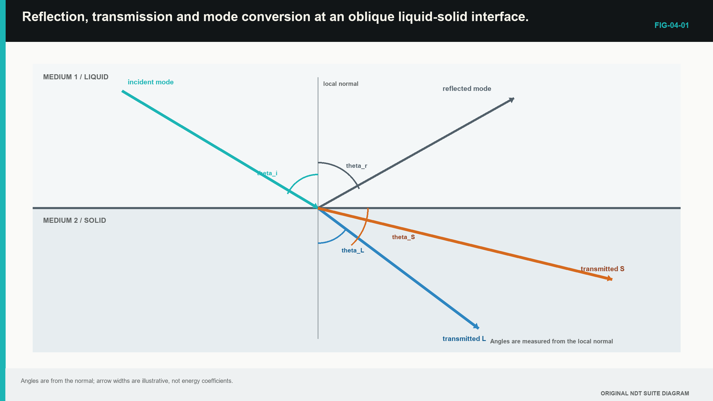
The normal is an imaginary line at 90 degrees to the interface. Unless a figure says otherwise, all incident and refracted angles in this book are measured from that normal.
For a flat interface between simple isotropic materials, Snell's relationship links the angle and speed on each side. In words:
sine of angle ÷ wave speed has the same value for matching ray components at the boundary
| (4.3) Snell relationship · EQ-04-04 Where: theta_1 = incident angle from normal; theta_2 = refracted angle from normal; c_1 = incident-mode speed (m/s); c_2 = refracted-mode speed (m/s) Model limits: planar interface, homogeneous isotropic media and phase velocities for mirror-like (specular) plane-wave components |
|---|
If the transmitted speed is higher, the transmitted angle is farther away from the normal. If it is lower, the path bends toward the normal.
A solid can support longitudinal and shear motion. An angled longitudinal wave entering a solid can therefore produce both a transmitted longitudinal wave and a transmitted shear wave. This is mode conversion. A liquid carries no ordinary bulk shear wave, yet a liquid-coupled longitudinal wave can still create shear inside a solid because the solid supplies shear stiffness.
The following figure shows the main ray families. Notice that arrow width is not an energy value and that all angles start from the normal.
| Worked example · Finding an incident angle for a 60-degree shear wave WE-04-02 Given: A wedge longitudinal speed is 2,330 m/s. Steel shear-wave speed is 3,230 m/s. The desired shear angle is 60.0 degrees from the normal. Find: The incident angle in the wedge. Steps: Rearrange Snell's relationship. sin(theta_w) = (2,330/3,230) sin(60.0 degrees) sin(theta_w) = 0.62472 Use inverse sine. theta_w = 38.7 degrees Answer: The estimated incident angle is 38.7 degrees from the normal. What this tells you: The result is a design estimate for the stated speeds and flat interface. Wedge wear, temperature, coupling and finite beam width affect the actual field. Common mistake: Measuring the 60-degree shear angle from the surface instead of from the normal. |
|---|
4.4 Critical angles and shear-wave wedges
Suppose sound travels from a slower wedge into faster steel. As the incident angle rises, the refracted angle rises faster. At one incident angle, a selected transmitted mode reaches 90 degrees and runs along the boundary in the simple ray model. This incident value is a critical angle.
In words:
critical incident angle = inverse sine of incident speed ÷ selected transmitted speed
| (4.4) Critical incident angle · EQ-04-06 Where: theta_c = incident angle at which the selected transmitted mode reaches 90 degrees; c_1 = incident-mode speed (m/s); c_2 = selected transmitted-mode speed (m/s) Model limits: c_1 < c_2; planar interface; homogeneous isotropic media; phase-velocity Snell model |
|---|
The first critical condition commonly refers to the transmitted longitudinal mode reaching 90 degrees. Above it, the simple model has no propagating transmitted longitudinal bulk wave. Shear may still propagate. At the second critical condition, the transmitted shear mode reaches 90 degrees.
Between those two incident angles, a wedge can favour a refracted shear wave in steel. The phrase “pure shear” is convenient but not exact. A real finite probe has angular spread and near-boundary fields. The established probe field matters more than a perfect line drawn in a notebook.
| Worked example · Estimating first and second critical angles WE-04-03 Given: Wedge longitudinal speed is 2,330 m/s. Steel longitudinal and shear speeds are 5,900 m/s and 3,230 m/s. Find: The first and second critical incident angles. Steps: Use EQ-04-06 for each transmitted mode. First critical angle: asin(2,330/5,900) = 23.3 degrees Second critical angle: asin(2,330/3,230) = 46.2 degrees Answer: The ideal estimates are about 23.3 degrees and 46.2 degrees from the normal. What this tells you: Between these values, the simple ray model retains a transmitted shear bulk wave but not a transmitted longitudinal bulk wave. A real beam changes over a region rather than at one perfectly sharp line. Common mistake: Using steel longitudinal speed for both critical-angle calculations. |
|---|
Step up preview - sensitivity near a critical angle
Near a critical condition, a small change in wedge speed, wear or incident angle can produce a larger change in the transmitted field. Level 1 therefore treats the calculated angle as a setup estimate and relies on a suitable reference check. The numerical sensitivity case moves to Level 3, where temperature and angle uncertainty are analysed formally.
4.5 Real contact surfaces and couplant layers
The equations so far describe flat, perfectly bonded interfaces. A hand-held probe meets something less polite. The surface has roughness. Couplant has thickness and viscosity. Pressure changes as the probe rocks. Curvature gives different local surface normals across the probe footprint.
Couplant is therefore a variable acoustic layer. If the layer becomes very thin and stable, it may act like an effective connection between the probe and component. As it thickens, its own travel time and multiple reflections can matter. Viscous material may remove more high-frequency content. Air pockets create strong local reflection.
Probe pressure can improve contact but can also change the layer thickness and contact footprint. On a curved pipe, the probe may contact only a narrow strip unless it has a suitable shoe. Curvature can redirect, focus or spread the transmitted field.
Reference comparison is strongest when the couplant, surface, temperature and pressure represent the component. A smooth block can confirm that the instrument and probe produce a reference response. It does not prove equal transfer through a rough corroded surface.
Surface roughness presents many small local angles. When roughness is tiny compared with wavelength, much of the field remains orderly. As roughness scale grows, more energy is scattered. A finite probe also contains a range of ray directions around its nominal centre. Near a critical condition, some parts of that range can support a mode while others do not.
4.6 Step up preview - coatings, bonds and very thin layers
A coating or bond layer has two close boundaries. When their echoes overlap, the layer may change response height and pulse shape without appearing as one separate peak. A weak interface echo therefore has more than one possible cause and must not be translated directly into a universal bond percentage.
Level 2 develops multiple reflections, interference, matching layers and representative bond specimens. The full thin-layer figure and treatment move with that topic; no thin-layer phase calculation is assessed in Level 1.
4.7 Free surfaces and strong corner responses
A free surface, such as a metal-to-air back wall, cannot carry normal contact force into the air in the same way as a bonded solid. The incident wave reflects strongly and can also change mode depending on angle and polarisation.
A right-angle corner can return a strong multi-bounce response toward the probe. A planar discontinuity meeting a back surface can create a useful corner-trap path. Normal root geometry, a counterbore or a cladding edge can create a similar strong response. Probe movement and geometry are needed to distinguish them.
The same strong peak can therefore have several causes. First compare its time with the known back wall or corner position. Then move the probe and see whether the response follows the expected geometry. A large response is useful evidence, but its height alone cannot tell the learner which corner produced it.
Step up preview - waveform sign and energy balance
Radio-frequency waveform sign and full reflected/transmitted energy accounting can help analyse an interface, but they require consistent polarity, coefficient definitions and every relevant mode. That formal treatment moves to Level 2 and Engineering Ultrasonics. Level 1 keeps the simpler rule that one received voltage is only part of the complete energy field.
4.8 Using the interface model without overclaiming
Every interface calculation should state:
- the incident and transmitted wave modes;
- the speed used for each mode;
- the angle convention;
- whether the surface is treated as flat;
- whether the material is treated as isotropic;
- whether the result describes amplitude, intensity or direction.
The calculation should then be compared with something measurable, such as a response from a known reflector, a refracted-angle check, an interface-echo time or a beam map.
In a direction-dependent material, the wavefront and the main energy path may point in different directions. The material can also support mixed wave patterns rather than one simple longitudinal or shear path. Curvature changes the surface normal across the probe, while coarse grains disrupt an orderly wavefront. Later levels call these effects quasi-modes, beam skew and aberration. The simple Snell calculation does not describe them. [R006]
The careful Level 1 statement is, “The calculated shear path is 60 degrees for the stated speeds and flat isotropic model.” It is not, “The beam is exactly 60 degrees everywhere because the wedge says 60.”
The interface and mode-conversion treatment used here follows the cited ultrasonic training and open wave foundations. [R001] [R004] The simple equations are valuable because they predict trends and allow nonsense checks. Their assumptions remain part of every result.
In plain words
- A boundary divides incoming sound among reflected, transmitted and sometimes converted modes.
- Acoustic impedance combines density and wave speed for a stated mode.
- A larger impedance mismatch normally produces stronger normal-incidence reflection.
- Angled sound refracts when wave speed changes across an interface.
- A solid can support mode-converted longitudinal and shear waves.
- Critical angles mark where a selected transmitted bulk-mode ray reaches 90 degrees in the simple model.
- Couplant, roughness, curvature and thin layers make real interfaces differ from ideal equations.
- A strong boundary response does not identify the reflector without geometry and movement evidence.
Key terms
- Interface: boundary between materials or material regions.
- Impedance: density multiplied by wave speed for the stated mode.
- Reflection: returned part of the incident sound.
- Refraction: direction change across a boundary.
- Mode conversion: creation of another wave mode at a boundary.
- Critical angle: incident angle at which a selected transmitted mode reaches 90 degrees in the simple model.
Key relationships
- Z = rho c: acoustic impedance combines density and speed.
- R_p = (Z2-Z1)/(Z2+Z1): ideal pressure reflection depends on impedance mismatch.
- sin(theta_1)/c_1 = sin(theta_2)/c_2: Snell's relationship links speeds and angles.
- theta_c = asin(c_1/c_2): a simple critical-angle estimate when the incident speed is lower.
Common mix-ups
- Pressure-amplitude and intensity coefficients are not the same quantity.
- Angles from the normal are not angles from the surface.
- Couplant improves the path but does not remove surface effects.
- A critical angle is not a perfectly sharp field boundary for a real finite probe.
- A strong corner echo is not automatically a crack.
Bridge to Chapter 5
This chapter followed sound across boundaries. Chapter 5 moves inside the probe and instrument chain. It explains how electrical energy becomes a pulse, how probe construction shapes that pulse, why cables and coupling matter, and how to choose a probe family for a task.
Sources and further study
- [R001]
- [R004]
- [R006]
CLASSROOM LAB · INTERACTIVE
Try critical angles
Change the incidence and watch the transmitted wave modes. This is a simplified teaching model, not a calibration or inspection calculation.
Open the full classroom lab ↗Study and revision only. This is not an approved inspection procedure, acceptance criterion or qualification.