
CHAPTER 51 · FMC / TFM / PCI Level 2
Seeing What Reconstruction Controls Change
In this chapter · 23 sections
Why this matters
The same FMC dataset can produce images that look coarse, smooth, bright, narrow, noisy or clean; some changes come from the numerical grid and display. Others come from the acoustic aperture, retained bandwidth and path support. Halving pixel spacing can make a response smoother without separating two targets. Independent normalisation can make a weak noisy view look as strong as a well-supported one. This chapter uses one dataset throughout so each control is changed visibly before the formal name, calculation and technique decision are introduced.
What you already need
- The Chapter 49 distinction between a calculated pixel and a physical reflector.
- The Chapter 50 requirement for a small set of justified path views.
- PAUT knowledge of aperture, frequency, bandwidth, filtering and encoded scanning.
- The ability to compare fixed-scale images and basic dimensions.
- Confidence with whole-number multiplication and simple rates.
What you will learn
- Separate pixel spacing from physical image resolution.
- Define a useful ROI and calculate its pixel count.
- Explain how aperture, bandwidth, filtering and normalisation change an image.
- Distinguish geometric, acoustic and encoded coverage.
- Estimate how reconstruction work grows with views, pixels and pairs.
- Build and freeze a basic Level 2 technique inside defined approval limits.
Words you will meet
- Resolution: demonstrated ability to distinguish separate features under a stated criterion.
- Pixel spacing: distance between neighbouring calculated image points.
- Point-spread response: finite reconstructed shape of a small target.
- Region of interest: declared component-coordinate area reconstructed as pixels.
- Normalisation: scaling values to a selected maximum or reference.
- Essential variable: a controlled setting whose change can affect the supported result.
- Sensitivity study: planned comparison that changes one input and measures its effect.
51.1 Reconstruct one dataset four ways
A verified teaching dataset contains two small reflectors separated by a known distance, one shallow target, one deep target and one target close to the lateral ROI boundary. The baseline uses a declared direct path, fixed aperture, 0.5 mm grid, no spatial smoothing and one fixed amplitude scale. The first copy changes pixel spacing to 0.25 mm. Edges look smoother and the peak coordinate changes slightly because the finer grid samples closer to the response maximum. The two close targets remain merged. Numerical sampling improved; demonstrated target separation did not.
The second copy restricts the aperture; the response broadens laterally and loses some coherent gain. A side feature decreases, but so does target support near the ROI edge. Calling that result cleaner would hide the trade. The third copy changes the frequency band. Background reduces, pulse shape changes and the apparent distance between overlapping peaks changes; the fourth copy independently normalises every view. All four now reach the same bright colour even though their absolute responses and noise margins differ.
This visible sequence establishes the chapter rule; a software control can change appearance, numerical sampling, acoustic evidence or all three. The technician measures the consequence instead of judging quality from polish. Published matrix-imaging material separates grid sampling, physical point response, aperture support and controlled display comparisons for the same reason. [R017] [R019] [R047]
51.2 Resolution has direction and a criterion
Resolution is the ability to distinguish separate reflectors or features under a declared test. Depth resolution concerns separation mainly along the local propagation direction and is strongly influenced by pulse duration and bandwidth. Lateral resolution concerns separation across that direction and depends strongly on wavelength, effective aperture, geometry and depth.
Orientation discrimination describes how the response changes as a reflector face rotates. Out-of-plane response describes how energy outside a nominal two-dimensional slice contributes; a one-dimensional linear array can produce a compact cross-sectional image while remaining broad in the passive elevation direction. The practical measurement is the point-spread response. Reconstruct a small representative target and measure response widths and side structure using a declared threshold and scale. Repeat the measurement at shallow, deep, central and edge locations; the result belongs to the complete probe, acquisition, material, path, ROI and processing arrangement.
A side-drilled hole is not an ideal point; a notch and a crack tip also scatter differently. The demonstration target is therefore evidence for its stated purpose, not a universal resolution token.
51.3 Pixel spacing samples the response
The grid asks the reconstruction calculation at separate coordinates. Coarse spacing can place the true peak between pixels; a small shift in probe or grid origin then changes which part of the oscillatory response is sampled. The image may look blocky and the displayed maximum may vary.
Fine spacing asks the same acoustic question at more locations; it improves smoothness and can reduce grid-placement error. It does not narrow the underlying point-spread response, increase source bandwidth or improve target orientation; it also increases processing, memory and the temptation to report unsupported decimal places.
The following figure places pixel squares over the same physical response; the important comparison is the response width and target separation, not the number of coloured squares.
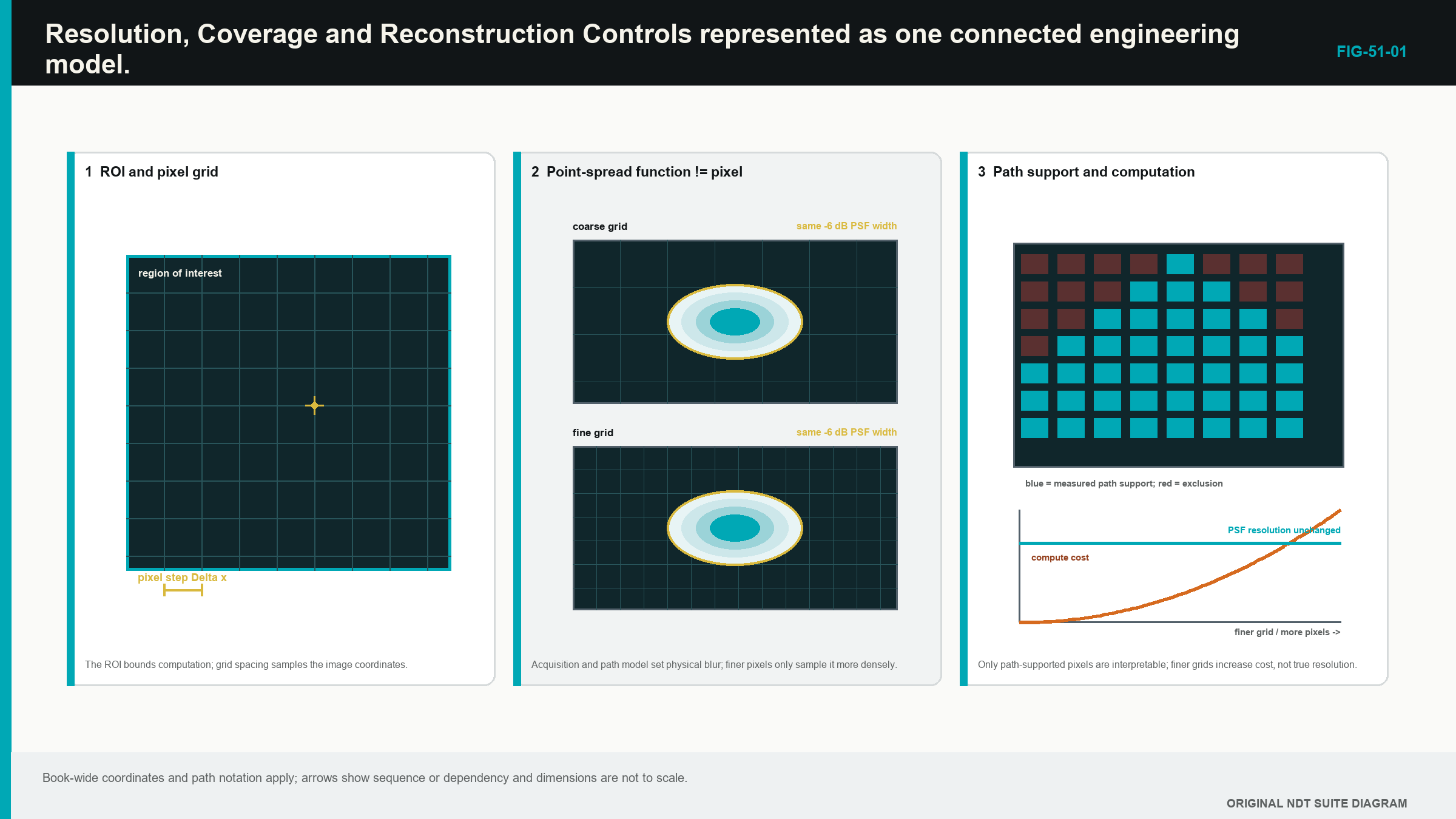
A wavelength fraction can provide a starting trial value; it is not a universal compliance rule. Signed RF, envelope and proprietary processing can respond differently to grid placement; the final increment is confirmed by measured position, response stability and separation performance.
51.4 Count the ROI before making it enormous
A rectangular ROI has a lateral span L_x, a depth span L_z, and positive increments Delta_x and Delta_z. If both endpoints are included, the number of points on each axis is the span divided by increment, rounded by the declared rule, plus one.
| (51.1) Pixel count on a rectangular reconstruction grid · EQ-51-01 Where: N_pix = reconstructed pixels per view (count); N_x = lateral grid points (count); N_z = depth grid points (count); L_x = lateral ROI span (m or mm); L_z = depth ROI span in the same unit; Delta_x = lateral increment in that unit; Delta_z = depth increment in that unit; floor(.) = round down to the next integer Model limits: a rectangular two-dimensional grid, both endpoints included and every x-z combination calculated |
|---|
The equation counts calculations; it says nothing about physical resolution or coverage. Software can also use a different endpoint convention, so setup transfer requires a reproduced boundary check.
| Worked example · Pixel count is not resolution WE-51-01 Given: A rectangular ROI spans 60 mm laterally and 40 mm in depth. Both endpoints are included and each axis uses 0.25 mm increments. Find: The number of grid points and total pixels. Steps: Lateral points are 60/0.25 + 1 = 241. Depth points are 40/0.25 + 1 = 161. Multiply them: N_pix = 241 x 161 = 38,801 pixels. Answer: The view contains 38,801 calculated pixels. What it means in practice: A finer grid increases coordinate sampling and computation, but target-separation performance still comes from the measured point response. Common mistake: Reporting 0.25 mm resolution because the pixels are 0.25 mm apart confuses numerical spacing with demonstrated acoustic resolution. |
|---|
51.5 Make the ROI follow the examination volume
The ROI begins and ends in declared component coordinates; it contains the required volume plus justified margins. It can be divided into zones when different paths support different regions. Overlaps show how one zone hands over to another. Wedge, air and physically impossible regions are excluded rather than coloured.
An ROI boundary can cut through a finite response and reduce its peak or apparent size. Demonstration therefore includes targets just inside important boundaries and checks the transition into adjacent zones. A target outside the calculated box should disappear from that view, but a response side lobe can still leak toward the boundary.
The acquisition time range must support the furthest path used anywhere in the ROI; the geometry model must also contain the real component surface and probe registration. A box extending beyond either support is an unverified calculation region.
The practical design uses the smallest region that contains the required task with suitable margins. Oversized canvases increase compute, encourage irrelevant artefacts and make it harder to see which path actually supports each area.
51.6 Change aperture and frequency with a purpose
The physical array provides possible elements; the effective aperture is the part that supplies useful transmit and receive geometry for a particular pixel. Central points may use a broad element range. Deep or lateral points can approach directivity and transmission limits, leaving fewer useful pairs.
Increasing aperture can narrow the main response laterally and improve coherent gain; it can also add poor-angle elements, model error, surface sensitivity and side structure. Restricting aperture can improve robustness or remove faulty channels, while broadening the response and reducing coverage elsewhere; the element range or pair rule is recorded explicitly.
Apodisation changes weights across the aperture; it can lower side lobes while widening the main response or reducing sensitivity. A generic window diagram does not establish the effect on the actual material and target.
Frequency and bandwidth begin with the probe, pulse, receiver and propagation. Higher frequency gives shorter wavelength but usually suffers more attenuation and scattering. Broader usable bandwidth can shorten a pulse and improve separation along the path. Reconstruction cannot restore frequencies not transmitted, received or retained.
A practical study compares central, edge, shallow and deep targets. One control changes at a time. Peak coordinate, response width, separability, background and repeatability are recorded together so improvement in one region cannot hide loss in another.
51.7 Keep filters, smoothing and normalisation visible
An acquisition filter acts before storage and can irreversibly remove content. A reconstruction filter acts on retained data and may be reversible when the full band survives. Either can change pulse shape, timing, phase, coherence and tip separation.
Acquisition averaging can reduce uncorrelated noise while the probe remains stationary. It lengthens the matrix cycle and can blur data if the probe moves. Spatial smoothing reduces pixel variation but can merge close features, lower peaks or fill gaps. Time interpolation, image interpolation and screen resizing are different operations and should not share one vague label.
Receiver clipping is source damage. Image saturation is a display limit. The first destroys waveform shape; the second paints several high calculated values with the same colour. Lowering the display range can reveal their differences only when the underlying values remain available.
Normalisation scales to a chosen maximum or reference. Per-image normalisation helps reveal pattern but prevents direct brightness comparison. A noisy unsupported view and a strong verified view can both reach 100 percent. Fixed reference-based scaling is needed for quantitative comparison, with the basis recorded.
Thresholding hides lower values; it does not remove them from the source data. A threshold can erase weak tips or split a broad response. Persistence and maximum hold can retain an earlier peak after coupling changes. Baseline and processed views are preserved separately.
51.8 Prove three kinds of coverage
Geometric coverage means a modelled route connects the aperture, region and receiver. Acoustic sensitivity means representative targets produce usable evidence throughout that region. Encoded coverage means physical scan positions sample the component without unacceptable gaps.
An ROI proves none of them by itself. A ray drawing supports geometry, not amplitude. A predicted sensitivity map depends on reflector and material assumptions. A central reference target does not prove edge or difficult-orientation performance. A fine encoded line does not compensate for poor through-wall path sensitivity.
Technique evidence therefore distributes targets through the required region and includes challenging orientations. It records near-surface, backwall-adjacent, central and lateral behaviour. Physical start, end and overlap marks test encoded extent. Unexamined areas remain visible.
When one view loses sensitivity near a boundary, another justified view or probe position may provide overlap. Making the original view brighter is not a coverage extension.
51.9 Understand the first-order computation scale
A straightforward reconstruction repeats pair processing for every pixel and every view. The first-order workload therefore grows with those three counts.
| (51.2) First-order reconstruction-work scale · EQ-51-02 Where: W = relative first-order reconstruction work; N_view = declared path views (count); N_pix = pixels per view (count); N_pair = retained contributing pairs (count) Model limits: comparable interpolation and per-pair processing; actual time also depends on software, hardware, memory movement and overhead |
|---|
Halving grid spacing in both axes gives roughly four times as many pixels in the same two-dimensional ROI. Doubling view count roughly doubles work. Moving from 32 by 32 ordered pairs to 64 by 64 gives four times the pair count. These multipliers combine.
The relationship supports planning, not a promised frame rate. Optimised software, graphics processing hardware, lookup tables and memory layout change actual performance. The technician measures witnessed valid position rate and watches for dropped data rather than relying on the screen refresh.
The best Level 2 setting is the coarsest grid and smallest justified workload that still meet location, stability, separation and coverage requirements with margin. More calculations are not a quality objective.
51.10 Begin a basic technique with the inspection problem
The technique brief identifies material, thickness, weld or component geometry, accessible surfaces, datum, temperature, coating and scan restrictions. It names the required detection, location, characterisation and sizing tasks separately. It also identifies target types, positions and important orientations.
Only then are probe, frequency, aperture and wedge selected. Probe clearance is checked on the real surface and scanner. The wedge and surface models include identity, wear, mounting and temperature limits. The acquisition plan states full or reduced matrix, pair population, sampling, range, gain, filters, stored signal type and encoder increment.
The reconstruction plan uses a limited path set from Chapter 50. Each view has a purpose, diagram, ROI, grid, aperture and demonstration target. Amplitude TFM and PCI controls remain separate. The amplitude plan records reference, gain, envelope and scaling. The coherence plan records implementation, band, aperture, thresholds and display range without inventing amplitude units.
An essential variable is a controlled input whose change can affect coverage, sensitivity, position, resolution, sizing, interpretation or traceability. Material, thickness, probe, wedge, matrix scheme, range, filters, encoder, velocity, path, ROI, grid, algorithm version and retained data can all be essential for a particular claim. A cosmetic window arrangement need not be essential when it cannot affect evaluation.
The Level 2 technician prepares and applies the defined plan inside its limits. New paths, changed algorithms, material outside the demonstrated range, unqualified sizing and missing acceptance criteria are approval gates for the designated technical authority.
51.11 Link scan speed to valid position rate
The scanner must allow the instrument to complete and retain the required data at each permitted increment. If scan speed is v_scan and the largest permitted position spacing is Delta_x, the valid complete-position rate must be at least their ratio.
| (51.3) Minimum encoded position rate · EQ-51-03 Where: f_position = valid complete acquisition positions per second (Hz); v_scan = scan speed (mm/s or m/s); Delta_x = maximum permitted encoded increment in the matching distance unit (mm or m) Model limits: steady motion, one complete dataset per accepted position and no missing, duplicated or silently interpolated positions |
|---|
At 60 mm/s with 1.0 mm maximum increment, the minimum is 60 positions/s. A witnessed system rate of 45 valid positions per second cannot support that speed and spacing. Slowing to no more than 45 mm/s gives the arithmetic limit before practical margin. The alternative is a separately demonstrated reduction in workload.
Display frame rate is not necessarily valid acquisition rate. The operator checks position count, dropped-data indicators and a trial scan at the planned speed.
51.12 Freeze a demonstrated setup
A controlled sensitivity study begins with one protected baseline. Pixel spacing, ROI origin, aperture, filter, smoothing and scaling are changed one at a time. The same shallow, deep, edge and close-target measurements are repeated. Peak position, response width, separation, background, processing time and file behaviour are recorded.
The selected setup is not the one with the smoothest image. It is the one that meets every declared task with margin and practical acquisition capacity. Rejected settings remain in the study, showing why they fail. The configuration is saved, closed, reopened and reproduced from the same data.
A completed weld-plan case then links component drawing, paths, acquisition, ROIs, domains, rate calculations, target evidence, essential variables and known limitations. The Level 2 technician can explain and follow that plan. Approval status remains explicit, and unresolved gates do not disappear into a footnote.
Formal multi-objective optimisation, pair-population design and computation release belong in Chapters 58 and 60. The Level 2 outcome is controlled comparison rather than algorithm design.
Step up
Chapter 58 develops grid, interpolation, computational precision and determinism. Chapter 60 treats acquisition-reconstruction co-design, coverage metrics and robust optimisation. Chapters 68, 72 and 80 provide the engineering treatment of point-spread functions, beamformer comparison and processing capacity.
In plain words
- Pixel spacing controls where the image calculation is sampled, not the width of the physical response.
- Resolution must state direction, target, location and the criterion used to separate features.
- The ROI should follow the required component volume and supported acoustic paths.
- Aperture and bandwidth affect real response, while normalisation and palette mainly affect presentation.
- Geometric, acoustic and encoded coverage are separate claims.
- Reconstruction work grows with views, pixels and contributing pairs.
- Scan speed and valid matrix rate must support the declared physical increment.
- A Level 2 technique freezes demonstrated controls and routes new design decisions for approval.
Key terms
- Resolution: demonstrated separation capability under stated conditions.
- Pixel spacing: distance between neighbouring calculated grid locations.
- Point-spread response: system-and-target image shape for a small reflector.
- ROI: bounded component-coordinate reconstruction region.
- Normalisation: scaling to a selected maximum or reference.
- Essential variable: controlled input capable of changing a supported result.
- Sensitivity study: one-change-at-a-time comparison of measured effects.
Key relationships
- N_pix = N_x N_z: axis point counts determine rectangular grid size.
- W proportional to N_view N_pix N_pair: views, pixels and pairs multiply first-order reconstruction work.
- f_position >= v_scan/Delta_x: valid complete-frame rate must support speed and encoded spacing.
- grid sampling != point response != target size: three distinct quantities must not be reported as one.
Common mix-ups
- A smoother fine-grid image does not prove two targets are resolved.
- A larger ROI does not create acoustic coverage.
- Fewer side features after aperture restriction do not prove overall performance improved.
- Per-image normalisation prevents direct brightness comparison.
- Display frame rate does not prove complete matrix acquisition rate.
Bridge to Chapter 52
Chapter 51 controlled amplitude reconstruction and the practical technique around it. Chapter 52 now introduces phase coherence from a repeating-wave picture. It explains what agreement means, why PCI can differ from amplitude TFM and where the phase evidence can fail before showing the formal coherence signpost.
Sources and further study
- [R017]
- [R019]
- [R047]
Study and revision only. This is not an approved inspection procedure, acceptance criterion or qualification.