
CHAPTER 3 · Ultrasonics Level 1
How an Ultrasonic Pulse Moves
In this chapter · 18 sections
Why this matters
Probe labels contain values such as 2.25 MHz or 5 MHz. Instruments display time in microseconds and distance in millimetres. Those numbers become useful only when the learner can picture what is moving. The component does not flow from the probe to the reflector and back. Its particles make tiny movements while a disturbance carries energy through the material. This chapter connects that physical picture to frequency, wavelength, pulse length, wave type, travel time and basic amplitude comparison.
What you already need
- Materials carry mechanical waves because they have mass and elastic stiffness.
- A pulse travels to a boundary and an echo can return.
- Pulse-echo distance uses an outward and return journey.
- Multiplication, division and powers of ten are explained in the examples.
What you will learn
- Describe wave travel without imagining material flowing through the component.
- Link cycle time, frequency, wavelength and speed.
- Recognise longitudinal, shear and surface-wave motion.
- Explain how pulse duration and bandwidth affect echo separation.
- Use travel time and decibel comparisons carefully.
- Recognise where the simple Level 1 wave model stops being reliable.
Words you will meet
- Frequency: number of cycles completed each second.
- Period: time taken for one cycle.
- Wavelength: distance occupied by one cycle in the material.
- Mode: a wave family defined by its pattern of motion.
- Bandwidth: the range of frequencies carried usefully by a pulse or system.
3.1 Cycles, frequency and period
Picture one tiny region inside a steel block. When an ultrasonic pulse arrives, that region moves a very small distance around its normal position. It pushes or pulls on the next region. The disturbance advances, but the particles remain in the component. Energy and information travel; the steel itself does not make a round trip.
The instrument repeats this event many times each second, but each firing is still a separate short pulse. One firing creates the outward journey. Returning sound from that firing creates the echoes. Keeping those events separate helps the learner distinguish frequency inside a pulse from the rate at which the instrument starts new pulses.
A repeated motion can be divided into cycles. One full cycle returns to the same stage of motion. The time for one cycle is the period, written T. The number of cycles completed each second is the frequency, written f.
Frequency is measured in hertz. One hertz means one cycle per second. Ultrasonic testing probes commonly work in megahertz. One megahertz, written MHz, is one million cycles per second.
Frequency and period describe the same repetition from opposite directions. More cycles per second means less time for each cycle. In words:
frequency = 1 ÷ period
| (3.1) Frequency and period · EQ-03-01 Where: f = frequency (Hz); T = period (s) Model limits: a periodic component represented by one period |
|---|
A 5 MHz component completes five million cycles each second. Its period is 1/(5 x 10^6) s, which is 0.2 microsecond. A real ultrasonic pulse is not an endless perfect cycle. It starts, rings for a short time and ends. The frequency still describes the oscillation carried inside that pulse.
The frequency printed on a probe is usually a centre or nominal value. A short pulse contains a range of frequencies. The printed number does not mean every part of the received waveform has exactly that frequency.
3.2 Wavelength and sound speed
Period describes one cycle in time. Wavelength describes one cycle in space. Imagine freezing a regular wave inside the material. The distance from one compression peak to the next matching compression peak is one wavelength.
Wave speed connects time and space. During one period, one cycle pattern advances by one wavelength. In words:
wavelength = wave speed ÷ frequency
| (3.2) Wave relationship · EQ-03-02 Where: lambda = wavelength (m); c = phase speed for the stated mode, direction and material (m/s); f = frequency (Hz) Model limits: linear propagation of a harmonic component in a medium represented by the stated speed |
|---|
For one wave type in a simple material, speed remains approximately constant over the normal probe band. If frequency doubles, wavelength halves. Higher frequency does not normally make that bulk wave travel faster. It changes the spatial scale of the oscillation.
This can be checked without seeing the microscopic motion. Use two suitable probes of different frequency on the same known block. Their back-wall echoes should arrive at about the same material time after their individual delays are corrected. Their pulse shape, height and noise can differ, but the steel has not assigned a new bulk-wave speed just because the probe label changed.
| Worked example · Wavelength at two probe frequencies WE-03-01 Given: Use a nominal longitudinal speed of 5,900 m/s. Compare 2.25 MHz and 5.00 MHz. Find: The wavelength at each frequency. Steps: Convert MHz to Hz and apply lambda = c/f. lambda_2.25 = 5,900/(2.25 x 10^6) = 0.00262 m = 2.62 mm lambda_5.00 = 5,900/(5.00 x 10^6) = 0.00118 m = 1.18 mm Answer: Wavelength is 2.62 mm at 2.25 MHz and 1.18 mm at 5.00 MHz. What this tells you: The higher-frequency wave has the shorter wavelength. That can support interaction with smaller features, but it does not guarantee better detection in a noisy or strongly attenuating material. Common mistake: Saying that the 5 MHz wave travels faster because its frequency is higher. |
|---|
Wavelength is not the same as beam width. It is also not a guaranteed minimum flaw size. Detection depends on pulse length, beam field, target direction, material noise and the response threshold as well as wavelength.
3.3 Different wave modes
A wave mode is a recognisable pattern of particle motion and field distribution.
In a longitudinal bulk wave, particles move mainly back and forth along the travel direction. This creates repeating compression and relaxation. Longitudinal waves can travel in solids and fluids.
In a shear bulk wave, particles move mainly across the travel direction. The material changes shape as the wave passes. An ordinary liquid does not maintain the shear stiffness needed for a freely travelling bulk shear wave.
A surface wave is concentrated near a free surface. Its motion contains both normal and sideways parts and becomes weaker with depth. Plates, pipes and shells can also carry guided waves whose motion spreads through their thickness.
The following figure exaggerates particle movement so it can be seen. Notice that the propagation arrow and particle-motion arrow point in different directions for a shear wave.
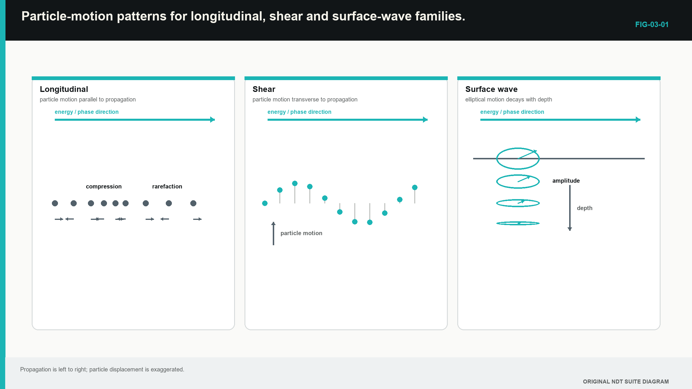
These families are simplified pictures. At an interface, one mode can create another. In directionally structured material, motion can be mixed. A shear wave also has a direction of particle movement, called polarisation. Those details become important in later levels.
For routine Level 1 calculations in fine-grained steel, we often treat one longitudinal or shear bulk mode as travelling at one speed along a straight path. That model is simple enough to use and strong enough to test against known reflectors.
A beginner can keep the two main bulk modes separate with one gesture. Point one hand along the travel direction. Move the other hand back and forth along that line for longitudinal motion. Move it sideways across the line for shear motion. The movement direction changes, so the material resistance and wave speed can also change.
3.4 A real pulse has length and bandwidth
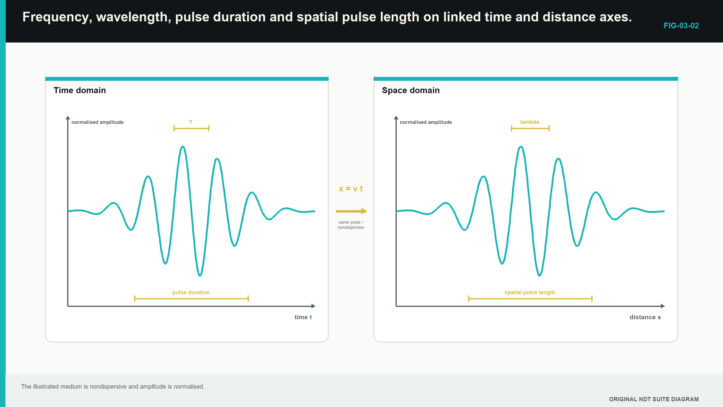
The probe does not produce one infinitely thin line. It produces a pulse that lasts for a short time. While the front of the pulse advances, the probe may still be completing later cycles. The pulse therefore occupies a length inside the material.
If a pulse contains n effective cycles and each cycle has wavelength lambda, its approximate spatial pulse length is n lambda. The same length can be found from wave speed multiplied by pulse duration.
In words:
spatial pulse length = speed × pulse duration = cycle count × wavelength
| (3.3) Approximate spatial pulse length · EQ-03-06 Where: SPL = spatial pulse length (m); c = wave speed (m/s); tau = effective pulse duration (s); n = effective number of cycles; lambda = wavelength (m) Model limits: weak dispersion and a representative speed and wavelength |
|---|
Two reflectors close together along the beam can return overlapping pulses. The display may then show one broad response rather than two separate responses. A shorter pulse generally improves the ability to separate them. This is called better axial resolution.
Imagine two thin flat boundaries at slightly different depths. The first echo has not finished before the second begins. Their voltages overlap on the screen and the pair may look like one wide peak. Increasing gain makes that combined peak taller, but it does not pull the two returning pulses apart. Pulse length must be addressed in the physical system.
Probe damping controls how quickly the element stops ringing. Strong damping normally gives a shorter pulse and broader bandwidth. Light damping allows more ringing and a narrower bandwidth. The strongly damped probe may separate close reflectors better, while the lightly damped probe may produce a higher narrow-band response. The best choice depends on the job.
| Worked example · Comparing two pulse lengths WE-03-04 Given: Shear-wave speed is 3,230 m/s at 4 MHz. Probe A gives an effective two-cycle pulse. Probe B gives an effective five-cycle pulse. Find: Centre wavelength and approximate pulse length for each probe. Steps: First find wavelength. lambda = 3,230/(4 x 10^6) = 0.0008075 m = 0.8075 mm Probe A: SPL = 2(0.8075) = 1.62 mm Probe B: SPL = 5(0.8075) = 4.04 mm Answer: Both probes have a centre wavelength of about 0.81 mm. Their approximate pulse lengths are 1.62 mm and 4.04 mm. What this tells you: Two probes with the same centre frequency can have very different echo-separation ability because their ringing differs. Common mistake: Using centre wavelength alone as a complete resolution value. |
|---|
The time and space views are linked in the following figure. Notice that frequency describes the cycles inside the pulse, while pulse duration describes the whole burst.
3.5 Travel time, distance and amplitude
For a known total travel path, time equals path divided by speed. In words:
travel time = total path ÷ wave speed
| (3.4) Travel time · EQ-03-05 Where: t = travel time (s); L = total travelled path (m); c = wave speed for the stated mode and model (m/s) Model limits: the path is represented by the stated length and effective speed |
|---|
Pulse-echo time normally includes the outward and return parts. If a total shear-wave path is already stated as 120 mm, do not divide it by two again. The path definition must be read before the calculator receives its ceremonial tapping.
| Worked example · Finding angle-beam transit time WE-03-02 Given: The total outward-and-return shear-wave path is 120 mm. Use a speed of 3,230 m/s. Find: The transit time. Steps: Convert 120 mm to 0.120 m and use t=L/c. t = 0.120/3,230 = 0.0000372 s t = 37.2 microseconds Answer: Transit time is 37.2 microseconds. What this tells you: An observed response near this time supports the proposed path. A large disagreement points toward a wrong path, wrong speed, wrong echo or uncorrected delay. Common mistake: Dividing the already stated total path by two. |
|---|
Amplitude can describe several physical quantities, including particle motion, pressure, stress or received voltage. The A-scan normally shows processed receiver voltage. It does not directly display acoustic energy at a discontinuity.
Decibels provide a convenient way to compare like amplitudes. For comparable voltage-like amplitudes, a drop to one-half is about -6 dB. A rise to twice the amplitude is about +6 dB. A tenfold amplitude rise is +20 dB. Level 2 develops the formal logarithmic equation and its use through a complete signal chain.
At Level 1, use decibels as a comparison label rather than a material-loss answer. If one echo is lower, first keep the probe, cable, gain, filter, gate and display view comparable. A gain change can make the screen height match while the physical received signal remains different.
Coupling gives a useful demonstration. Rock a probe slightly on a known block and watch the back-wall height change. The material did not suddenly absorb more sound. The contact path changed. This shows why a decibel difference needs a controlled comparison before it is assigned to the component.
The formal logarithmic calculation and the squared-amplitude example move to Level 2. No Level 1 assessment requires a learner to enter a logarithm. The beginner should recognise the common half-amplitude and double-amplitude reference changes and state what was kept the same.
3.6 Step up preview - why pulse shape can change
Two wave movements can add when they share the same place and time. Matching parts can strengthen each other, while opposite parts can reduce the immediate result. This is why a raw radio-frequency (RF) waveform can change after a very small probe movement even when the overall echo remains in the same region.
A short pulse also contains a range of frequencies. The probe, material, cable and receiver can change that mixture as the pulse travels through the system. Level 3 and Engineering Ultrasonics develop phase, interference, Fourier description, spreading and group velocity. Level 1 uses one representative speed only where the returned pulse and known path support that simple model.
3.7 Step up preview - how a digital instrument records a pulse
A digital instrument records the electrical waveform as separate samples and uses them to draw the A-scan. A smooth display is therefore a representation of recorded points, not proof of infinite detail. More screen pixels cannot recover information that the physical pulse and probe never captured.
Level 2 explains sample rate, anti-alias filtering and the different algorithms that can choose a pulse time. Those topics are not assessed as Level 1 mathematics in this progression. For now, retain the waveform and its settings whenever a reported value needs to be checked.
3.8 Using the simple model honestly
The Level 1 model works well when one bulk mode travels through a reasonably uniform material over a useful frequency band. It uses one representative speed and a clear path. Several common mistakes arise when that model is extended too far:
- Higher frequency does not normally make a nondispersive bulk wave travel faster.
- Gain does not shorten a pulse or narrow a beam.
- Wavelength is not beam width.
- Probe centre frequency is not the only frequency in a pulse.
- A stored velocity is an input until it has been supported by a known path.
- A tiny image pixel is not proof of equally tiny physical resolution.
- Equal display height does not mean equal reflector size or equal acoustic energy.
When waveform shape changes strongly with path, the time feature used for measurement must be named. When the material is anisotropic or a guided mode is dispersive, phase and energy can follow different directions or speeds. Those cases need later models rather than forced use of the simple one.
The bulk-wave, pulse-echo and wave-mechanics foundations in this chapter follow the cited open ultrasonic and wave teaching sources. [R002] [R004]
In plain words
- Particles make tiny movements while the ultrasonic disturbance travels through the material.
- Frequency counts cycles per second; period is time per cycle.
- Wavelength is one cycle measured through space.
- In a simple material, raising frequency shortens wavelength rather than raising bulk-wave speed.
- Longitudinal and shear waves have different particle-motion directions.
- Pulse duration and ringing affect whether nearby echoes can be separated.
- Travel time, amplitude and decibels describe different parts of the signal.
- Sampling and timing algorithms represent the waveform; they do not create unlimited resolution.
Key terms
- Frequency: cycles per second.
- Period: time for one cycle.
- Wavelength: distance for one cycle in the material.
- Mode: wave family with a particular motion pattern.
- Bandwidth: useful frequency range of the pulse or system.
- Phase: position within a cycle.
Key relationships
- f = 1/T: frequency and period are reciprocals.
- lambda = c/f: wavelength equals speed divided by frequency.
- SPL = c tau = n lambda: pulse length follows duration or effective cycle count.
- t = L/c: travel time equals total path divided by speed.
Common mix-ups
- Frequency is not speed.
- Wavelength is not beam width.
- Centre wavelength alone is not axial resolution.
- Gain changes displayed amplitude, not physical resolution.
- A dB change in received voltage does not identify one physical cause.
Bridge to Chapter 4
This chapter followed a pulse through one material. Real inspections contain boundaries: probe to couplant, couplant to component, weld regions, coatings, cracks and back walls. Chapter 4 explains why some sound returns, some crosses and some changes direction or mode at those boundaries.
Sources and further study
- [R002]
- [R004]
Study and revision only. This is not an approved inspection procedure, acceptance criterion or qualification.