
CHAPTER 18 · Ultrasonics Level 3
From Following a Technique to Controlling a Measurement System
In this chapter · 21 sections
Why this matters
A Level 2 technician can set up a proven angle-beam technique, establish its references, complete the scan and interpret the expected responses. The Level 3 problem begins when one part of that arrangement changes, or when somebody asks what the demonstration actually proves. A replacement wedge may carry the same nominal angle while moving the beam, delay and sensitivity. A block may contain ten clear notches while the production population contains rough natural cracks, several operators and variable surfaces. Level 3 work turns those practical observations into a bounded technical claim that can survive change, review and time.
What you already need
- The Level 2 separation between detection, location, characterisation, sizing and evaluation.
- Basic angle-beam geometry, calibration and reference-sensitivity concepts.
- The practical effects of probe, wedge, cable, coupling, gain and scan position.
- The difference between a repeatable observation and an acceptance decision.
- Confidence using algebra and simple squared-root calculations.
What you will learn
- Define the complete ultrasonic measurement system around a decision.
- Turn a broad inspection request into separate performance claims.
- Explain an essential variable through its causal effect on performance.
- Separate demonstrated evidence, model assumptions and unsupported extension.
- Analyse a change without automatically repeating everything or accepting everything.
- Build an uncertainty and evidence argument that includes people, software and records.
Words you will meet
- Measurement system: every controlled part that can influence the reported ultrasonic result.
- Performance claim: a precise statement of what the system can establish under stated conditions.
- Target population: the range of components and discontinuities to which the claim is intended to apply.
- Essential variable: a variable whose change can alter a supported performance claim.
- Applicability domain: the conditions inside which evidence supports use of a model or technique.
- Human factor: a feature of human work or work design that can change performance.
- Uncertainty: incomplete knowledge about a value, model, population or decision.
- Change impact: the route by which a proposed change affects evidence and outputs.
- Provenance: the retained identity and history of data, processing and configuration.
Depth guide for this chapter
- Understand here: the system boundary, causal variables, evidence boundaries and change logic.
- Calculate here: a conditional uncertainty combination and simple impact comparisons.
- Derive later: formal mathematics for shared variation, sensitivity matrices and advanced uncertainty propagation are developed in Chapter 64 and Chapter 78.
18.1 The familiar Level 2 problem
Consider a validated manual angle-beam technique used on ferritic welds; the procedure names a 45-degree probe, a reference sensitivity, scan positions and a recording rule. The original wedge is damaged, so the stores team supplies another wedge marked with the same nominal angle. A Level 2 setup reveals a different delay, a slightly different index point and a small sensitivity change; the technique can still be calibrated, but calibration alone does not show that its original coverage and detection evidence remain valid.
Level 2 knowledge already supplies the important observations; wedge delay moves the time origin. Index position changes the relationship between probe position and beam entry, refracted angle changes the beam path, and insertion loss changes the response relative to the reference. Level 3 reasoning connects each observation to the claim that depends on it; that connection is the beginning of technical control. The same logic applies when nothing has obviously broken; a successful demonstration on a reference block is useful evidence, but its meaning depends on material, thickness, targets, access, operator, equipment and decision rule. A result can be technically correct within that set and still be unsafe to extend outside it; Level 3 does not reject practical demonstrations, but states what each demonstration supports.
18.2 From a technique to a complete system
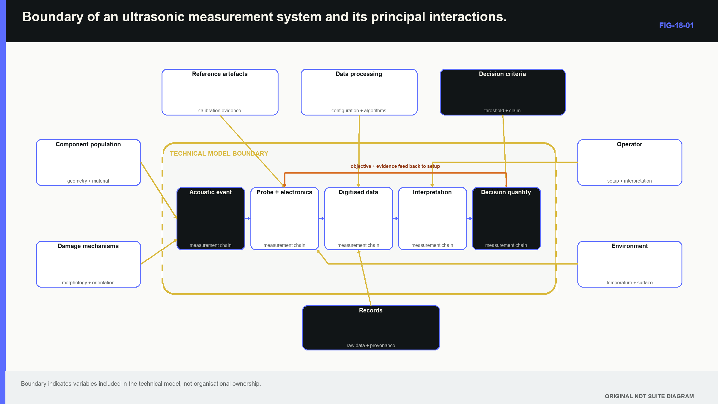
A technique is often discussed as a list of settings and scan positions; a measurement system is wider. It includes the component population, credible damage mechanisms, equipment, software, probe, wedge, cable, coupling, scanner, environment, reference artefacts, analyst, decision rule, data processing and records, and each part can change the result or its meaning. The system boundary should be drawn around every influence material to the claim; it does not describe organisational ownership. For example, an analyst may belong to another department, but analysis remains inside the technical system when interpretation affects the reported outcome. The governing acceptance criterion may be supplied by a client, yet it remains part of the decision model.
The following figure places the instrument inside this larger boundary; notice that the instrument is one link rather than the whole system.
One useful formal description treats the reported output as the result of inputs passing through a declared model.
| (18.1) Generic measurement model · EQ-18-02 Where: y = reported measurand or decision quantity; x_i = measured or assigned input quantities; M = declared physical and processing model; g = relationship mapping inputs to output Model limits: all influential inputs and model choices material to the claim are identified |
|---|
In plain language, g is the set of relationships used to turn observations into a result; for angle-beam depth, inputs can include transit time, zero, velocity, angle, probe index and selected echo. The model M states that a particular mode followed a particular path to a particular reflector; the equation supports dependency tracing but does not prove that every input or the chosen echo is correct.
18.3 Begin with the decision and credible damage
Technique design starts with the engineering information needed, not with available equipment; the output may be detection, location, through-wall height, remaining ligament, classification or a screening result. These outputs require different evidence. A technique that detects a strong response may still lack the resolution or signal identity needed for sizing. The next input is the credible damage mechanism; a damage mechanism describes how service, manufacture or material condition could create the target. Fatigue cracking may produce tight planar surfaces with preferred orientation. Casting shrinkage may be volumetric and distributed. Corrosion changes a boundary and makes spatial sampling important. The mechanism shapes the target population used for technique design and demonstration.
A target population includes more than size; it includes location, orientation, roughness, morphology, closure, surrounding material structure and relevant component variation. A 3 mm-deep machined notch and a 3 mm-deep natural crack share a dimension but not necessarily an acoustic response. The demonstration target must therefore be described as evidence for a class, not renamed as the whole class. Beginning with the decision prevents familiar equipment from defining the problem; it also reveals trade-offs. High gain may help detection while raising false calls. A narrow focused field may improve local response while losing robustness to position or velocity. The Level 3 task is to choose and defend the balance required by the decision.
18.4 Requirements, claims, evidence and assumptions
A requirement states the outcome needed; a performance claim converts that requirement into something that can be tested. Evidence is the observation or study supporting the claim. Assumptions connect demonstrated conditions to intended use. The applicability domain is the boundary inside which those connections remain defensible. The five familiar ultrasonic jobs should remain separate in the claim structure:
- Detection claims describe the target and probability or demonstrated sensitivity.
- Location claims describe the coordinate quantity and expected error.
- Characterisation claims describe supported categories and confusion risks.
- Sizing claims define the physical dimension, method, bias and spread.
- Evaluation claims identify the governing rule and decision boundary.
Combining them into “the technique is qualified” hides important differences; a system may detect reliably but overestimate height. It may locate well in homogeneous plate but become biased through directional weld metal. A classifier may work for represented geometries and fail on an unseen configuration. Each claim needs its own inputs, evidence and limit. Public general-principles standards organise method concepts without supplying every application’s scan extent or acceptance rule. [R041] Certification curricula also organise the knowledge expected at different levels, including modern ultrasonic methods, but they do not make one person or one technique universally authorised. [R060] The project requirement and the physical performance argument must remain connected and distinct.
| Worked example · Unpacking a broad detection claim WE-18-01 Given: A mechanised angle-beam technique detected ten 3 mm-deep electro-discharge-machined notches in one 25 mm ferritic-steel plate. All notches were perpendicular to the scanning surface and examined by one operator. Find: The part of a broader detection claim supported by this evidence. Steps: Define the demonstrated domains for material, thickness, target type, orientation, surface, equipment configuration, operator and sample size. Compare each domain with the proposed production population. Mark every untested extension as an assumption rather than evidence. Answer: The trial supports detection of those ten high-contrast notches in that plate and configuration by that operator. It does not establish population probability of detection (POD), natural-crack performance, other orientations, other material structures, operator variability or different thicknesses. Technical implication: The result is useful feasibility evidence. A broader claim requires representative targets, controlled variation and an appropriate reliability design. Common mistake: Reporting ten successes as proof of certain detection for every 3 mm crack changes a bounded observation into an unsupported population claim. |
|---|
18.5 Essential variables are causal variables
An essential variable matters because its change can affect a performance claim; the term is not created merely by placing an item on a controlled list. Frequency can change wavelength, attenuation and pulse duration. Aperture can change beam width and side-lobe structure. Surface preparation can change coupling. Scan increment can create spatial gaps. Software can change filtering, measurement or data interpretation.
The causal route should be stated; a new cable may change delay and spectrum but leave component geometry untouched. A replacement wedge can change delay, index, angle, field and insertion loss. A new material heat can change velocity, attenuation and structural noise. A new display scale can change human recognition without changing stored radio-frequency data. These changes do not deserve identical tests because they do not touch identical claims.
Controlled flexibility is more useful than either extreme; freezing every detail can make a technique brittle and prevent technically equivalent substitution. Allowing wide ranges without evidence makes the original demonstration meaningless. A justified range is supported by tests across the range, a physical model with confirming observations, or both. Change analysis follows four steps:
- Measure or describe what changed.
- Link the change to affected system outputs.
- Identify the earlier evidence supporting those outputs.
- Repeat, bridge or retire only the evidence that no longer applies.
This sequence produces targeted re-evidence; it does not turn change control into an automatic full requalification, and it does not accept nominal labels as proof of equivalence.
18.6 Failure modes and the human contribution
Failure-mode thinking traces how a plausible-looking result can still be wrong; the chain can be divided into excitation, propagation, interaction, reception, processing, interpretation and decision. Weak excitation can reduce sensitivity. The assumed path can miss the target. Structural noise can mask an interaction. The receiver can saturate. Processing can remove evidence. An analyst can associate a response with the wrong geometry. A correct measured dimension can then be compared with an obsolete rule.
The important failure modes depend on consequence, likelihood and how easily they are detected; a weak reference response that appears in a routine check is different from silent beam skew that produces a convincing response at the wrong coordinate. The silent error deserves stronger development evidence because the normal stability check may not reveal it. People are part of the system; scanning consistency, fatigue, workload, display design, prior information and decision incentives can influence performance. Expertise remains valuable, but a system that works only through undocumented expert habits is difficult to reproduce. Encoded position, retained raw data, stable analysis sequences and peer review make expert contribution more observable.
Blind trials and independent interpretations can estimate human variation; a second reading of the same case is not fully independent if the first result is known. Prior geometry information can help an analyst form the correct hypothesis, while a previous call can anchor the result. The work design should state when context is provided, when independence is required and how disagreement is preserved.
18.7 Technical decision case: substituting a wedge
The opening Level 2 problem can now be treated as a complete change-impact case.
| Worked example · Assessing a wedge substitution without repeating unrelated evidence WE-18-02 Given: A validated angle-beam system is proposed to receive a new wedge of the same nominal angle. The probe and instrument are unchanged. Measured wedge delay changes by 0.18 microseconds, probe index moves 1.4 mm, refracted angle changes from 45.2 degrees to 47.0 degrees, and insertion loss changes by 0.6 dB. Find: The evidence claims directly affected by the substitution. Steps: Map delay to range origin. Map index and angle to beam intersection, location and coverage. Map insertion loss to reference sensitivity and amplitude comparison. Check whether instrument timing, digitiser resolution, operator competence or component population changed independently. Answer: Renew zero, index and angle characterisation. Revise coverage and coordinate calculations. Confirm sensitivity transfer. Retain existing instrument-linearity evidence when configuration identity shows the instrument is unchanged. Repeat application demonstrations only where the changed field or path no longer represents the original evidence. Technical implication: A nominally identical wedge is neither automatically acceptable nor a reason to repeat every unrelated test. The measured causal changes determine the evidence response. Common mistake: Correcting delay and then treating beam location as unchanged ignores the measured index and angle differences. |
|---|
This case contains three levels of decision; understanding identifies which physical outputs changed. Calculation updates delay, coordinates and coverage. Derivation of the underlying sensitivity matrix is not required here. Chapter 64.12 develops sensitivity matrices, called Jacobians, and Chapter 78 develops formal uncertainty and reproducibility treatment.
18.8 Uncertainty has more than one layer
Level 2 repeat readings often reveal spread; Level 3 must also examine model and population uncertainty. A practical structure has three layers:
- Measurement uncertainty describes incomplete knowledge of values while a chosen model is held fixed.
- Model uncertainty describes uncertainty about the path, mode, echo identity or relationship used.
- Population uncertainty describes how well demonstrated components, targets, operators and environments represent intended use.
These layers should not be hidden inside one unexplained plus-or-minus number; repeating cursor placement can reduce uncertainty in selecting the same peak while doing nothing to show that the peak is a crack tip. A second physical view or movement study addresses model identity. More representative specimens and operators address population support. When one model M is fixed and a local small-change approximation, known as linearisation, is adequate, correlated input contributions can be combined formally.
| (18.2) Conditional combined standard uncertainty · EQ-18-01 Where: u_c(y | M) = standard uncertainty in output y conditional on model M; c_i = local output sensitivity, expressed as the partial derivative of g with respect to input x_i; u(x_i,x_j) = covariance, a measure of how inputs i and j vary together Model limits: model identity is fixed, local linearisation is adequate and input covariance is represented |
|---|
The observable supported by this equation is a standard uncertainty for output y under one declared model; it can support comparison with a measurement tolerance or a change in uncertainty. It cannot legitimise an unresolved echo assignment. The notation y | M keeps that boundary visible. At this level, the learner should understand why shared errors can move inputs together and why covariance matters; the learner should be able to use supplied sensitivity and covariance values. Derivation of partial derivatives, covariance matrices and repeated random-sampling methods known as Monte Carlo alternatives belongs in Chapter 64 and Chapter 78.
18.9 Evidence through the system life cycle
The evidence argument changes over time; development establishes feasibility. Characterisation measures influential behaviour. Demonstration tests representative cases. Routine verification checks selected indicators of continued condition. Incident review investigates unexpected outcomes. Change control identifies which evidence survives modification. Retirement occurs when equipment, software or references can no longer sustain the claim. Routine checks are smaller than qualification because they answer a different question; a reference echo can show that selected system features remain stable. It cannot recreate a population reliability study. Conversely, repeating a full reliability study every day is neither practical nor necessary when sensitive condition indicators are identified.
Records preserve the link; a screen image without calibration state, raw-data identity or coordinate convention may look persuasive and remain technically weak. A reference response without probe identity or software version cannot establish comparability. Recording every field without a retrieval model creates volume rather than knowledge. Useful provenance retains enough context to reconstruct the measurement claim. The international ultrasonic training foundation connects principles, equipment, calibration, technique and interpretation. [R001] Level 3 extends that connection into an evidence system that can be challenged and maintained. Its mature statement names the population and decision, the supporting evidence, the controlled variation and the signals that reveal loss of validity.
18.10 Formal depth and the Part VIII handoff
Part III requires the learner to design the reasoning, interpret supplied uncertainty calculations and recognise unsupported inference; it does not assume an engineering degree. The complete mathematical tools are deliberately staged later:
- Chapter 64.8 introduces correlation, covariance and causation.
- Chapter 64.12 develops Jacobians and propagation through coordinate models.
- Chapter 78.1 defines the measurand formally.
- Chapters 78.2, 78.3 and 78.12 develop uncertainty evaluation, nonlinear propagation and variance components.
Those chapters derive and extend the models; this chapter establishes why the models are needed and which decision they support.
In plain words
- Level 3 work begins when a defined technique must be justified, changed or defended.
- The instrument is one part of a measurement system that also includes component, person, processing and decision rule.
- Detection, location, characterisation, sizing and evaluation need separate performance claims.
- Evidence supports only the conditions and populations it represents.
- An essential variable matters because it has a causal route to a supported output.
- Change control follows affected claims rather than labels such as minor or identical.
- Measurement, model and population uncertainty answer different questions.
- Provenance preserves the technical meaning of evidence as the system changes.
Key terms
- Measurement system: all controlled influences that create and interpret the result.
- Performance claim: testable statement of capability within stated conditions.
- Target population: components and targets to which the claim is intended to apply.
- Essential variable: variable whose change can alter performance or evidence validity.
- Applicability domain: bounded conditions supported by evidence.
- Human factor: human or task feature that influences system performance.
- Uncertainty: incomplete knowledge about value, model, population or decision.
- Provenance: identity and history needed to reconstruct evidence.
Key relationships
- y = g(x_1, ..., x_n; M): a reported output depends on inputs and a declared model.
- u_c(y | M): combined standard uncertainty is conditional on the selected model and represented covariance.
- change -> affected output -> supporting evidence: causal tracing defines targeted re-evidence.
Common mix-ups
- A successful demonstration is evidence, not proof for every production population.
- An essential variable is not made essential by a list alone.
- Repeatability does not resolve a wrong path or wrong echo identity.
- A routine reference check does not recreate qualification evidence.
- Nominally identical equipment does not prove task-linked equivalence.
Bridge to Chapter 19
Chapter 18 treated the physical model as one declared part of the system; most Level 2 work uses a scalar velocity, a familiar beam direction and a simple path. Chapter 19 shows how to recognise the symptoms that make that model inadequate, then adds only the wave physics needed to choose better evidence.
Sources and further study
- [R001]
- [R041]
- [R060]
Study and revision only. This is not an approved inspection procedure, acceptance criterion or qualification.