
CHAPTER 41 · Phased Array Ultrasonics Level 3
Calibration as Trustworthy PAUT Measurement
In this chapter · 27 sections
Why this matters
A reference echo returns to the same amplitude after calibration, yet its indicated position is wrong and the error changes across the sector. The amplitude check did its job; it was asked to prove something it cannot prove. PAUT calibration is a family of controls for timing, wedge behaviour, sensitivity, law response, encoder scale and component coordinates. Metrology is the discipline of making those measurements trustworthy and stating how uncertain they remain. This chapter begins with visible repeated readings and bias, then builds the measurement model, uncertainty budget, assurance checks and calibration-state record expected from a PAUT Level 3.
What you already need
- Level 2 PAUT calibration for velocity, wedge delay, sensitivity, TCG and encoder distance.
- The difference between indication amplitude, time, sound path and component coordinate.
- Basic mean, range, standard deviation and root-sum-square combination.
- Focal-law, coordinate-transform and automation dependencies from Chapters 38–40.
- The practical uncertainty introduction from UT Level 2 and Level 3 foundations.
What you will learn
- Define metrology and the quantity being measured in plain practical terms.
- Separate timing, velocity, wedge, sensitivity, encoder and application evidence.
- Build and interpret a PAUT coordinate uncertainty budget.
- Distinguish repeatability, reproducibility, bias and stability.
- Select checks that are sensitive to the failure being controlled.
- Maintain a calibration state through changes, drift and abnormal events.
Words you will meet
- Metrology: work of making measurements trustworthy and comparable.
- Measurand: the particular quantity intended to be measured.
- Traceability: documented connection from a result to references through calibration steps.
- Bias: systematic tendency for a result to differ from reference truth.
- Standard uncertainty: uncertainty expressed on a standard-deviation scale.
- Sensitivity coefficient: change in an output caused by a unit change in one input.
- Correlation: shared variation between input quantities or results.
- Reproducibility: variation when relevant conditions such as operator or system change.
- Stability: change in measurement behaviour with time.
- Measurement assurance: evidence that the valid measurement state continued during work.
41.1 Begin with readings that disagree in different ways
Place a known reflector at several sector angles and repeat the scan after removing and replacing the probe. Suppose peak amplitude stays within 0.5 dB, but the displayed x-coordinate is consistently 1.2 mm high at large angles and repeated remounting adds 0.4 mm scatter.
Three ideas are already visible. The repeat readings have spread. The large-angle results have a systematic offset, or bias. The behaviour changes with angle, so one constant correction is unlikely to describe the complete model.
Metrology is not a laboratory badge attached to this exercise. It means defining the result, understanding what changes it, comparing it with suitable references and reporting what the evidence supports. The first step is to name the quantity. “Calibration” is too broad; “component x-coordinate of a stated reflector under the released law set” is testable.
The following figure separates the main input paths to PAUT coordinate and amplitude results.
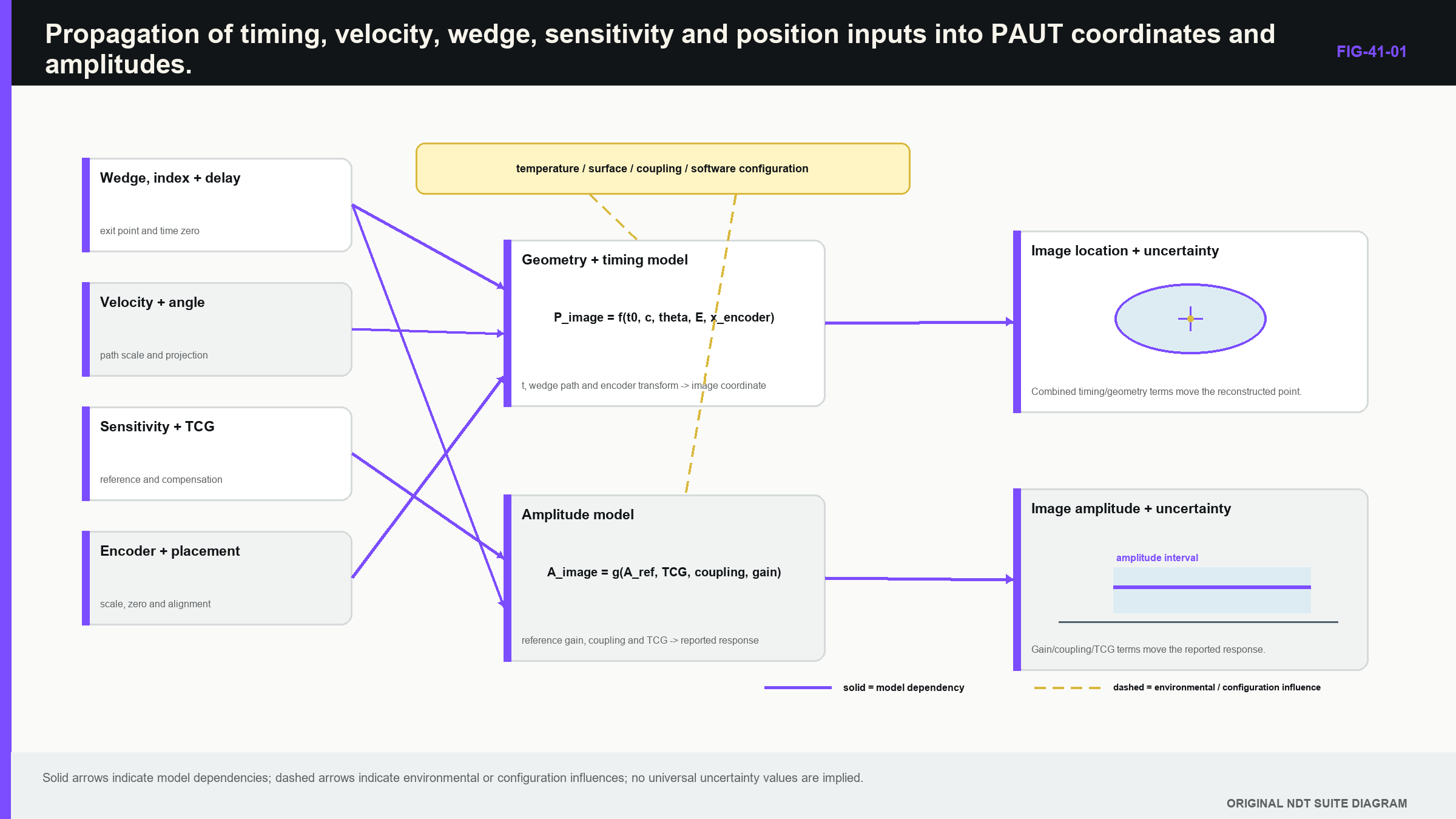
Notice that reproducing one amplitude does not establish the timing and coordinate branch of the measurement.
41.2 Define the measurand and measurement model
The measurand is the specific quantity intended to be reported. It may be reflector depth, component x-coordinate, remaining wall, response amplitude relative to distance-amplitude correction (DAC), encoder distance or a tip-to-tip height. Each requires a different model and reference chain.
An indicated coordinate can depend on sample time, channel delay, wedge geometry, wedge velocity, material velocity, refracted path, element location, probe placement and encoder position. A comparative amplitude can depend on target response, coupling, aperture, element sensitivity, gain, TCG, filtering and normalisation.
Write the model before listing uncertainties. The list should follow how the result is actually calculated. A tidy budget containing every familiar calibration item can still be wrong if it omits signal identity or double-counts one shared correction.
International uncertainty guidance treats uncertainty as a property of a stated model and conditions. [R031] [R032] It does not provide one universal PAUT accuracy. The Level 3 task is to connect each input to the output, justify its estimate and retain the evidence that defines the present configuration.
41.3 Traceability is a chain with a limited purpose
Traceability links a result to references through documented calibration steps, each with uncertainty. Not every field adjustment is a metrological calibration in the strict sense. Some operations standardise a setup or check function. Naming them correctly helps stop one reference response from being promoted into proof of the whole technique.
A controlled block dimension can support time or length scale. Instrument clock performance may support timing. Amplitude is usually comparative and belongs to the complete acoustic chain. Velocity can be measured on the component, estimated from a representative coupon or taken as a bounded model input.
The reference object has dimensional tolerance, material variation, surface condition and reflector geometry. A certificate describes some properties; it does not remove transfer error. A precisely known hole in dissimilar fine-grained steel can establish distance scale while remaining poor evidence for attenuation, scattering or planar-target sensitivity in a coarse weld.
Traceability strength must be output specific. State which property the reference supports, which uncertainty it contributes and where transfer to the component becomes an assumption.
41.4 Separate offset, scale and angular error
For a direct pulse-echo distance, velocity error changes scale and delay error adds an offset. In a wedge and sector path, errors also depend on element and angle. Aligning one reflector with one delay can hide residual error elsewhere.
In words, a small distance change contains contributions from velocity, measured time and reference delay. The first-order relationship is:
| (41.1) First-order distance sensitivity to velocity and timing · EQ-41-02 Where: delta_d = small change in reported distance (m); c = represented velocity (m/s); t = measured round-trip time (s); t0 = reference delay (s); delta_c = small velocity change (m/s); delta_t = small measured-time change (s); delta_t0 = small delay change (s) Model limits: direct homogeneous pulse-echo model; small perturbations; correct echo identity; first-order linearisation around the stated operating point |
|---|
The equation identifies different signatures. A constant delay change moves shallow and deep results by a similar distance. A velocity change creates error that grows with path. Angle or wedge-shape errors can create direction-dependent residuals not represented by the simple equation.
Temperature changes wedge and component velocity and can change wedge dimensions. Wear changes height, angle and contact. A single correction is useful only within its demonstrated range. Targets at several depths, lateral positions and angles help separate coupled parameters that one target cannot identify.
41.5 Sensitivity standardisation is not field repair
Sensitivity standardisation establishes a comparative response using a declared target, path, law, aperture, focus, coupling and processing chain. Law-to-law correction can compensate predictable response differences, but it can also hide a weak law if gain is unlimited.
Review reserve gain, noise and saturation with the correction. TCG changes gain with time, increasing later noise as well as the reference. DAC changes the comparison curve. Digital normalisation and colour maps can make laws look equal without changing raw signal-to-noise ratio.
A reference family does not make service reflectors equivalent. Cylindrical holes, notches and planar cracks have different directivity. Extrapolating a correction beyond its measured range adds model uncertainty. Interpolation rules and raw recoverability should be stated when amplitude supports a decision.
Failure case: equalised poor law. One maximum-angle law needs 14 dB more correction than its neighbours and leaves only 2 dB headroom before clipping on strong geometry. The equalised reference image looks uniform. The underlying law has poor field support or transmission and may not meet detection or artefact claims. Investigation, redesign or a narrowed law range is more defensible than further gain.
41.6 Encoder and coordinate calibration
Encoder calibration estimates scale, direction and repeatability over representative travel. Component coordinates also depend on scan origin, probe offset, skew, surface model and registration. Correct encoder scale plus wrong probe offset gives a perfectly repeatable displaced dataset.
Raster scans need scan and index evidence. Manual index steps, mechanical stops and a second encoder have different error models. Curved components may use arc length, angle or developed distance; a flat view is not automatically Cartesian truth.
Use features whose coordinates are known independently of the PAUT setup. Repeat in both directions to expose slip and backlash. Compare ultrasonic response coordinates with external positioning evidence to separate acoustic-path error from scanner error.
Change case: updated surface model. Raw encoder positions and waveforms remain unchanged, but a revised nozzle surface changes component coordinates by up to 1.5 mm. Encoder calibration remains supported. Component registration and any coverage or sizing output based on the old model require change-impact review.
41.7 Build the uncertainty budget after seeing the errors
An uncertainty budget lists the inputs in the actual measurement model. Repeated measurements can estimate some components. Certificates, resolution, specifications and prior data support others. The traditional Type A and Type B labels describe how an estimate was made, not its importance.
Each input uncertainty is converted to its effect on the output by a sensitivity coefficient. Independent contributions combine by root-sum-square. Shared inputs create correlation and require covariance terms.
| (41.2) Combined standard uncertainty including correlation · EQ-41-01 Where: u_c(y) = combined standard uncertainty of output y; c_i = sensitivity coefficient for input i; u_i = standard uncertainty of input i in its units; corr_ij = correlation coefficient between inputs i and j Model limits: the model is adequately linear over the stated uncertainty range; included inputs represent material sources; coefficients and correlations apply to the declared configuration |
|---|
The observable is the uncertainty scale of a named output, not general technique quality. Correlation can increase or reduce the uncertainty of a combination. Two tip depths using the same velocity may move together, so their height difference can cancel part of the shared scale error.
41.8 Worked coordinate budget
| Worked example · Build a simplified location-uncertainty budget WE-41-01 Given: A nominal 50.0 mm shear-wave distance uses 3,230 m/s. Standard relative velocity uncertainty is 0.5%. Equivalent round-trip timing uncertainty is 20 ns. Probe-index uncertainty projected onto the reported coordinate is 0.20 mm. Treat the three contributions as independent for this simplified case. Find: The combined standard uncertainty for the stated coordinate model. Steps: Velocity contribution is 50.0 mm x 0.005 = 0.25 mm. Timing contribution is 3,230 m/s x 20 x 10^-9 s / 2 = 0.0323 mm. Combine: u_c = sqrt(0.25^2 + 0.0323^2 + 0.20^2) mm = 0.322 mm. Answer: Combined standard uncertainty is approximately 0.32 mm for the included terms. Technical implication: Velocity and projected probe-index terms dominate this simplified budget. Angle, wedge geometry, surface, target localisation, reader choice and correlation remain outside it. Common mistake: Reporting 0.32 mm as universal PAUT coordinate accuracy or adding percentage, time and distance values before converting them into the same output unit. |
|---|
A sense check compares the result with its largest component. Root-sum-square of independent terms must be at least as large as the largest contribution, 0.25 mm, and smaller than their simple sum, 0.482 mm. The calculated 0.32 mm lies inside that range.
41.9 Repeatability, reproducibility and stability
Repeatability uses closely repeated conditions. Reproducibility changes relevant factors such as operator, probe, instrument, day or analysis implementation. Stability looks for change with time. Ten readings without remounting can be tightly grouped while probe replacement produces much larger variation.
Study factors that the intended process allows. Include replacement if replacement is permitted. Include readers if boundary selection is manual. Include systems if they are claimed equivalent. A balanced or nested design can separate components when enough observations exist.
Control charts can show drift, but statistical and technical limits differ. A point inside a broad statistical limit may already threaten a coordinate tolerance. One point outside a narrow statistical limit may be technically harmless. Establish the action rule from both process behaviour and measurement consequence.
Evidence-boundary case. A study shows excellent same-operator repeatability on polished blocks, but production involves rough surfaces, probe remounting and two analysts. The study supports only the narrow conditions tested. It cannot be used as the reproducibility component for production without additional evidence.
41.10 Design checks around the failure to be detected
Instrument, probe and complete-system checks control different functions. A passing instrument check does not prove an array or wedge. Standards scopes reflect these layers, and complete-system imaging checks do not automatically prove application performance. [R043] [R044] [R045] Public guidance similarly distinguishes characteristic evaluation from application calibration. [R049]
A useful check is sensitive to the relevant fault, repeatable enough to see meaningful change and practical at the required interval. Element maps can reveal weak or dead channels. Reference targets can reveal timing and sensitivity drift. Encoder travel can reveal scale or slip. None proves faults outside its design.
When a check fails, investigate rather than immediately restore the number. Identify affected times, laws, groups and outputs. Preserve the failed state and find the last known valid point. Recalibration after repair proves current performance; it does not validate earlier data unless the fault boundary is supported.
41.11 Correlation, nonlinearity and signal identity
Calibration creates correlation. Velocity estimated from reference times may later be used to locate both tips. A common delay may move every depth. The uncertainty calculation should follow the same dependency graph as the result.
First-order coefficients work when small input changes stay on one path and select the same echo. Near a path branch, mode transition or peak-selection change, the output can jump. A single symmetric standard deviation then hides multiple possible results.
Signal identity can be categorical. A weak response may be an upper tip, geometry or another mode. This is not simply an extra 0.5 mm of coordinate uncertainty. Retain conditional interpretations and sizes until evidence resolves the category.
Monte Carlo simulation can carry nonlinear models and common inputs when distributions are defensible. Preserve joint samples so correlation survives. Inspect skew, multiple modes and reference-truth coverage, not only final standard deviation.
41.12 Validate the budget against observed performance
A budget should predict repeatability and reference error across its intended range. Systematic underprediction points to missing components, incorrect distribution or wrong correlation. Extreme overprediction can occur when broad specification limits are treated directly as standard uncertainties.
Version the budget with probe, path, calibration method, target family, software and reader process. Changing one can change sensitivities and distributions. Copying the previous uncertainty number into a new technique is not propagation.
For amplitude, keep electronic repeatability, coupling, target placement, transfer and correction-curve uncertainty distinct. Convert dB and linear amplitude quantities consistently. Adding percentage and decibel standard deviations is dimensionally meaningless.
Expanded uncertainty uses a coverage factor under a stated interpretation. It is not a convenient guard band. The governing decision process decides how uncertainty affects acceptance; the NDT result provides the value, uncertainty and basis. [R031] [R032]
41.13 Maintain a calibration state through the scan
Calibration establishes a state at one time. Measurement assurance shows that the state remained valid during work. Use pre-, intermediate and post-checks according to drift risk, temperature, wear, scan duration and consequence.
Continuous indicators such as interface response, element energy or encoder health can narrow the affected interval after a fault, but only when their relationship to the measurement function has been demonstrated. A healthy interface echo may not prove coordinate transform or law timing.
Assign a calibration-state identifier after the dependent set passes. Attach it to acquired data until a change, failure or expiry creates another state. Any adjustment during scanning creates a new state, requires dependent checks and marks a dataset boundary.
Quietly changing gain or delay without a state transition destroys traceability. A post-check does not reveal the exact drift history; it only helps bound it. Record the evidence and any assumption used to accept or reject the interval. [R031] [R032] [R043] [R044] [R045]
41.14 Reporting boundaries honestly
A calibration result states measurand, model, reference chain, configuration, value, uncertainty and conditions. It separates standardisation or functional checks from traceable calibration where appropriate.
Where the reference does not represent component attenuation, anisotropy or target directivity, say so beside the result. A traceable distance can remain valid without becoming proof of detection. An amplitude standardisation can remain useful without proving a natural crack response.
The Level 3 release question is whether each reported quantity can be traced to a current calibration state and an uncertainty model whose most important contributors have been tested. If the answer is limited, narrow the measurement claim rather than enlarging a single convenient tolerance.
41.15 End-to-end case: a coordinate passes one check and fails another
A sector is standardised on a side-drilled hole near the middle of its angular range. The reflector depth repeats within 0.3 mm. A second reflector near the high-angle boundary is then reported 1.4 mm too far in x while its depth remains within 0.5 mm. The instrument timebase and encoder scale both pass their separate checks.
The pattern points away from one global length-scale error. Candidate contributors include wedge geometry, probe index, angular law delay, refraction model and component transform. The useful response is to compare observed error against angle and coordinate, then perturb those inputs in the measurement model. A constant x-offset suggests registration. Error that grows with steering suggests an angular, delay or wedge-model term.
Suppose independent wedge metrology finds wear concentrated beneath one side of the aperture. Recalculated laws and reference measurements reduce the high-angle x bias to 0.4 mm across the released range. The calibration state is then rebuilt with the new wedge identity, law checksum, timing results, reference scans and uncertainty budget.
Earlier data do not automatically inherit the corrected state. The impact review uses the last known geometry condition, scan dates, intermediate checks and the sensitivity of each reported coordinate to the worn region. Where that evidence cannot bound the effect, location claims are withdrawn or the component is rescanned.
This case connects metrology to governance. A passing central reflector proved a limited timing and coordinate case. The high-angle failure exposed a model term outside that evidence. The corrected result becomes trustworthy only after the dependent functions, uncertainty and dataset boundary are all updated together.
The retained record also separates reference-truth uncertainty from PAUT scatter. If the high-angle reflector position is known only within 0.2 mm, that contribution enters the comparison rather than disappearing behind the larger observed bias. Repeating the case with a second reference orientation checks whether the correction follows wedge geometry or has merely been tuned to one target. The release range is the set of angles and coordinates challenged by those independent references, not every law that the instrument can display.
41.16 Design measurement assurance around drift mechanisms
Measurement assurance is strongest when each indicator responds to a known failure mechanism. Temperature can change wedge delay and velocity. Wear changes geometry and coupling. Connector or channel degradation changes amplitude and phase. Encoder slip changes spatial scale. Software state can change coordinates without altering the raw echo.
For a long automated weld scan, begin with the outputs that matter. Detection may depend on comparative sensitivity and element condition. Location depends on timing, velocity, law identity, registration and encoder state. Tip height also depends on boundary selection and correlated coordinate errors. One intermediate reference response cannot observe every path.
Build a small assurance set with complementary sensitivity. A stable reference echo challenges selected acoustic timing and amplitude. An interface or coupling indicator can reveal contact change. Sequence and encoder diagnostics challenge data association. Configuration checksums and coordinate regression cases challenge digital state. Their intervals follow how quickly each mechanism can change and the consequence of delayed detection.
Suppose an interface amplitude drifts gradually while a high-angle reference time remains stable. The evidence points toward coupling or surface behaviour rather than one global clock change, but it does not prove field support everywhere. If an encoder scale check then fails, the coordinate interval is bounded independently from the amplitude interval.
After a fault, assurance data can narrow impact only within demonstrated sensitivity. A healthy central target cannot clear a high-angle wedge-wear mechanism that it scarcely samples. A software checksum can prove the executable identity while remaining silent about a misplaced scanner origin.
The final plan names each indicator, measurement function, threshold or trend rule, interval, retained evidence and response. This turns pre- and post-checks into a designed observation system and prevents one convenient echo from becoming a ceremonial certificate for unrelated quantities. [R031] [R032] [R043] [R044] [R045] [R049]
Trend limits should be based on observed stability and decision consequence, not copied automatically from a specification tolerance. A small consistent drift can reveal a developing mechanism before the final tolerance is exceeded. Conversely, ordinary remounting scatter should not create repeated false alarms. Baseline data, control-chart logic where suitable and periodic review keep the assurance rule connected to real system behaviour.
In plain words
- Calibration is a family of measurement controls, not one reference echo set to a chosen height.
- Metrology means making a named measurement trustworthy and stating what remains uncertain.
- Timing, velocity, wedge, sensitivity and encoder controls support different outputs.
- Repeatability, reproducibility, bias and stability reveal different weaknesses.
- An uncertainty budget must follow the actual calculation and preserve correlation.
- A passing instrument check does not prove the probe, wedge or application.
- A failed check starts impact investigation; a later adjustment does not validate earlier data automatically.
- Every dataset should remain linked to the calibration state under which it was acquired.
Formal synthesis
PAUT calibration becomes metrology when it begins with a measurand and a transparent measurement model. Traceability and standardisation have output-specific boundaries. First-order sensitivities, covariance and observed variation convert input knowledge into a coordinate or amplitude uncertainty, while nonlinear path and signal-identity cases require conditional treatment. Measurement assurance, calibration-state identity and failure-impact analysis keep the model connected to data throughout the inspection interval.
Key terms
- Metrology: discipline of trustworthy, comparable measurement.
- Measurand: the exact quantity intended to be reported.
- Traceability: documented calibration chain to references.
- Bias: systematic difference from reference truth.
- Sensitivity coefficient: output response to an input change.
- Correlation: shared input or output variation.
- Measurement assurance: evidence that the valid state continued during work.
Key relationships
- EQ-41-02 separates first-order velocity, measured-time and delay contributions to distance change.
- EQ-41-01 combines uncertainty contributions and their correlations for one declared output.
- Independent contributions combine by root-sum-square only after conversion into the output unit.
- Shared errors can cancel in a difference even while they remain in absolute coordinates.
Common mix-ups
- Repeatability is not accuracy.
- Traceable reference dimension is not representative target response.
- Law equalisation is not restoration of missing field support.
- Encoder calibration is not complete component registration.
- Expanded uncertainty is not a universal acceptance guard band.
Bridge to Chapter 42
Chapter 41 established trustworthy measurement states and uncertainty. Chapter 42 uses those foundations to qualify a complete PAUT technique. It begins with a bounded performance claim and follows one continuing case through model evidence, representative specimens, robustness, blind confirmation, transfer and technical review.
Sources and further study
- [R031]
- [R032]
- [R043]
- [R044]
- [R045]
- [R049]
Study and revision only. This is not an approved inspection procedure, acceptance criterion or qualification.