
CHAPTER 13 · Ultrasonics Level 2
Angle-Beam Geometry and a Practical Coverage Plan
In this chapter · 20 sections
Why this matters
A ray can pass neatly through the centre of a weld on paper while the real scan misses an important region. The probe may not fit at the required position. The angle may be different from its label. Beam width changes with depth, and a planar target may face away from the beam. Level 2 coverage planning joins calculation to the real component. This chapter builds one weld plan step by step, then tests it against access, orientation, scan spacing and encoded data rate.
What you already need
- Angle is measured from the local surface normal in this book.
- Sound path, depth and surface distance can be found with basic trigonometry.
- Probe index is the acoustic exit reference on the scanning surface.
- A central ray represents only the centre of a finite field.
- Actual thickness and actual refracted angle are needed for useful geometry.
What you will learn
- Establish a clear component coordinate system.
- Calculate a probe position for a first-leg target.
- Relate fusion-face direction to a useful beam direction.
- Add access, probe footprint, beam width and scan spacing to a ray plan.
- Include longitudinal and transverse target orientations.
- State uncovered or conditional regions honestly.
Words you will meet
- Datum: the chosen reference from which coordinates are measured.
- Skew: rotation of the beam direction across the scanning surface.
- Fusion face: the prepared joint face intended to fuse during welding.
- Coverage: supported ability to examine a stated region and target class.
- Occlusion: a region blocked by geometry or another acoustic boundary.
- Raster scan: parallel scan lines covering an area.
- Overspeed: motion too fast for the required data spacing.
13.1 Draw the component before drawing the beam
Begin with the as-built component, not an idealised weld symbol. Record actual wall thickness, weld centreline, bevels, root face, cap profile, backing, mismatch, attachments and accessible surfaces.
Choose a datum that can be found again. In a simple plate weld, x can run across the weld, y along the weld and z downward from the scanning surface. The probe index has an x and y position. Skew states the surface direction in which the beam points.
The coordinate convention should be visible on the drawing and record. A response at “42 mm” has little meaning without stating whether 42 mm is sound path, depth, surface coordinate or distance from weld centreline.
For the recurring weld case, use a 20 mm plate with a single-V weld, meaning that the two prepared sides form a V-shaped joint. The scan surface is the top of the plate. The first coverage check is whether the chosen beam can reach the root, both fusion faces and the required weld volume from accessible positions.
13.2 Place a first-leg ray at a target
For a straight first-leg model, the horizontal offset from the probe index to a target is depth multiplied by the tangent of the refracted angle.
In words:
probe position = target surface coordinate minus the horizontal beam offset
| (13.1) Probe position for a first-leg target · EQ-13-02 Where: x_probe = probe-index coordinate; x_target = target surface coordinate; z_target = target depth; theta = refracted angle from normal Model limits: two-dimensional straight first-leg ray and declared positive direction | (13.1) Probe position for a first-leg target · EQ-13-02 Where: x_probe = probe-index coordinate; x_target = target surface coordinate; z_target = target depth; theta = refracted angle from normal Model limits: two-dimensional straight first-leg ray and declared positive direction |
|---|---|
| Worked example · Place the probe for a fusion-face point WE-13-01 Given: A target point is 12.0 mm deep at surface coordinate 40.0 mm. Use a 60.0-degree first-leg ray directed in positive x. Find: The required probe-index coordinate. Steps: Find the horizontal offset. x_offset = z tan(theta) = 12.0 mm x tan60 degrees x_offset = 12.0 x 1.732 = 20.8 mm Subtract the offset from the target coordinate. x_probe = 40.0 - 20.8 = 19.2 mm Answer: Place the probe index at approximately 19.2 mm in the declared coordinate frame. What it means in practice: The central ray now passes through one target point. The wedge footprint, beam width, target direction and surface access still have to be checked. Common mistake: Using the front or back of the wedge instead of the established probe index. |
The same calculation can be repeated for the root, upper fusion face and other important locations. Plotting several rays begins to show which probe positions are required.
13.3 Match the beam to target direction
A smooth planar reflector normally gives its strongest pulse-echo return when the beam is near normal to its face. A fusion face therefore needs more than a ray that crosses it. The direction of the beam relative to the face matters.
Draw the face and its normal. Compare the beam with that normal. Do not compare a probe label with a bevel label without first checking how each angle is measured.
Real lack of fusion can be wavy. Cracks can curve. A range of angles is often more useful than one perfect nominal angle. The purpose of several probes or scan directions is to add target-orientation evidence, not merely fill the report with familiar numbers.
Volumetric pores and rough reflectors scatter more broadly, although their responses can still vary with angle. Tip diffraction can also return energy over a wider direction range than a smooth face, but tip responses are usually weaker.
13.4 Add skip paths and probe access
The first-leg ray reaches the back wall after a path set by thickness and angle. Its horizontal travel to the back wall is the half-skip distance. After reflection, the second leg returns toward the top surface. Full skip is twice the half-skip surface distance for a parallel plate model.
These points help place the probe for root and fusion-face paths. They also reveal whether the wedge can physically reach the position.
Add the complete wedge outline to the drawing. A weld cap, attachment, edge or curved surface can block the position even when the index point appears clear. The scanner may also need travel beyond the nominal scan region so the acoustic exit point reaches the boundary.
Actual thickness matters. A thicker local region shifts skip positions. Mismatch can place the root differently from the nominal drawing. A useful plan includes the range of as-built geometry that the technique is expected to cover.
13.5 Replace the line with a finite beam
The central ray shows a plausible path. Beam width shows a region of response around that path. Near-field variation, focus and divergence make the width change with depth.
The coverage figure below combines several finite beam envelopes with weld geometry. Notice the difference between a ray touching a region and a supported beam envelope covering it.
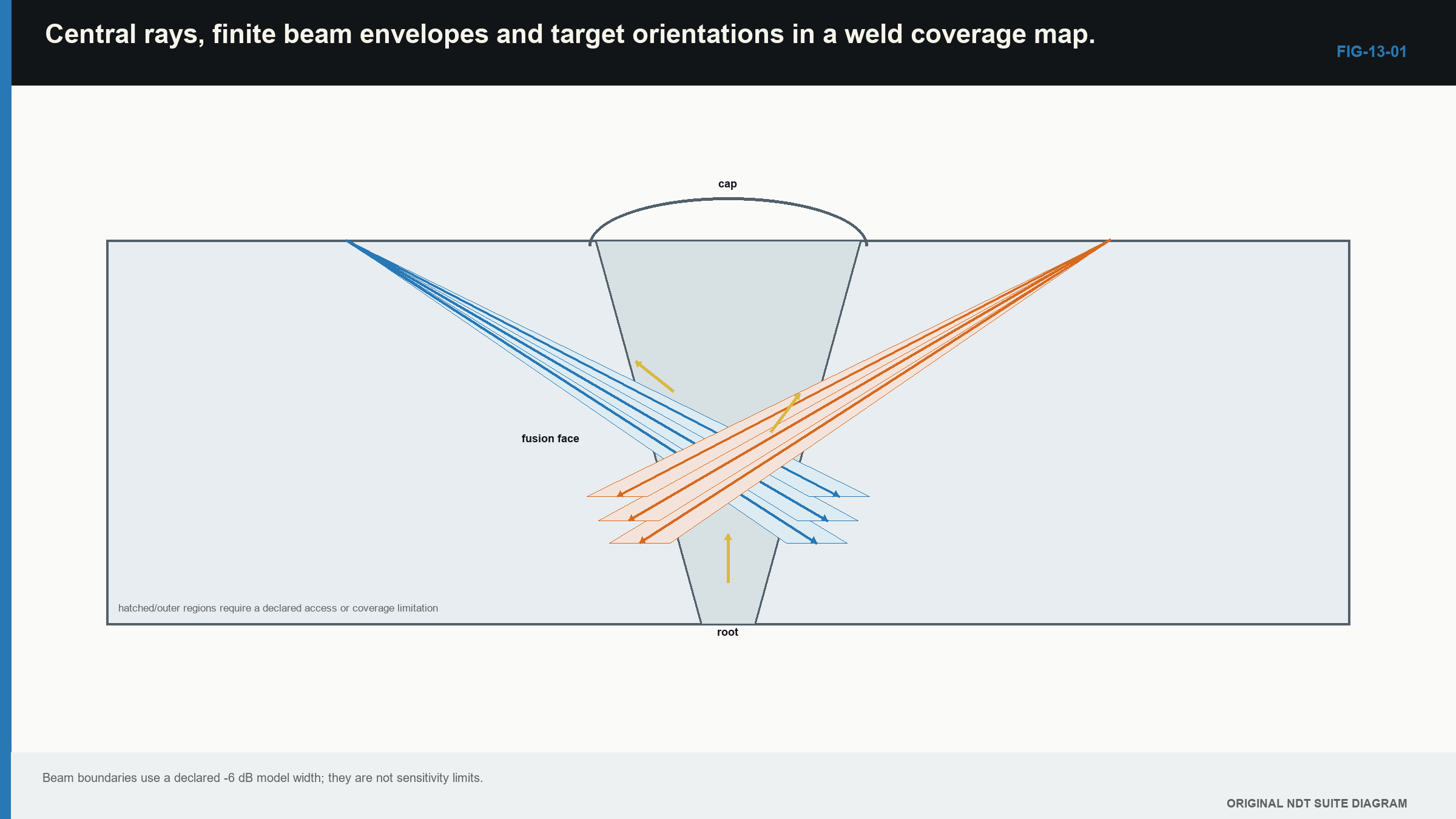
A 6 dB beam contour is not a wall. Sensitivity falls gradually, and target response changes with direction. Use the contour as a planning convention supported by representative targets.
Multiple depths should be checked. A scan pitch suitable at the focal depth may leave gaps where the beam is narrower elsewhere. The weakest target orientation or deepest region deserves representative evidence.
13.6 Choose scan-line spacing
For a raster or parallel-line scan, track spacing should be related to measured beam width at the target depth. The next example uses a simple overlap calculation.
| Worked example · Calculate nominal overlap between scan lines WE-13-02 Given: Measured 6 dB beam width at the target depth is 8 mm. Scan-line spacing is 6 mm. Find: Nominal overlap at that contour. Steps: Subtract spacing from width. overlap = 8 mm - 6 mm = 2 mm Convert to a fraction of the stated width. overlap fraction = 2/8 = 0.25 Answer: Nominal overlap is 2 mm, or 25%, at the stated depth and contour. What it means in practice: This is one coverage input. It does not prove detection between tracks because target direction and local sensitivity also matter. Common mistake: Applying the 25% value at every depth without checking how beam width changes. |
|---|
Manual scanning adds probe-placement variation. Encoded scanning records position more consistently, but only when encoder scale, direction and traction are correct.
13.7 Cover transverse as well as longitudinal targets
A scan perpendicular to the weld is well placed for many fusion-face and longitudinal discontinuities. It may give poor incidence on a transverse crack.
Skewing the probe or scanning along the weld adds a beam component in the weld-length direction. The convention for positive skew must be stated. The physical wedge footprint and cap shape can limit the available rotation.
Target orientation and spatial position are two different coverage questions. A beam may reach the whole weld volume while remaining poorly aligned with one crack direction. The orientation figure below shows both ideas together.
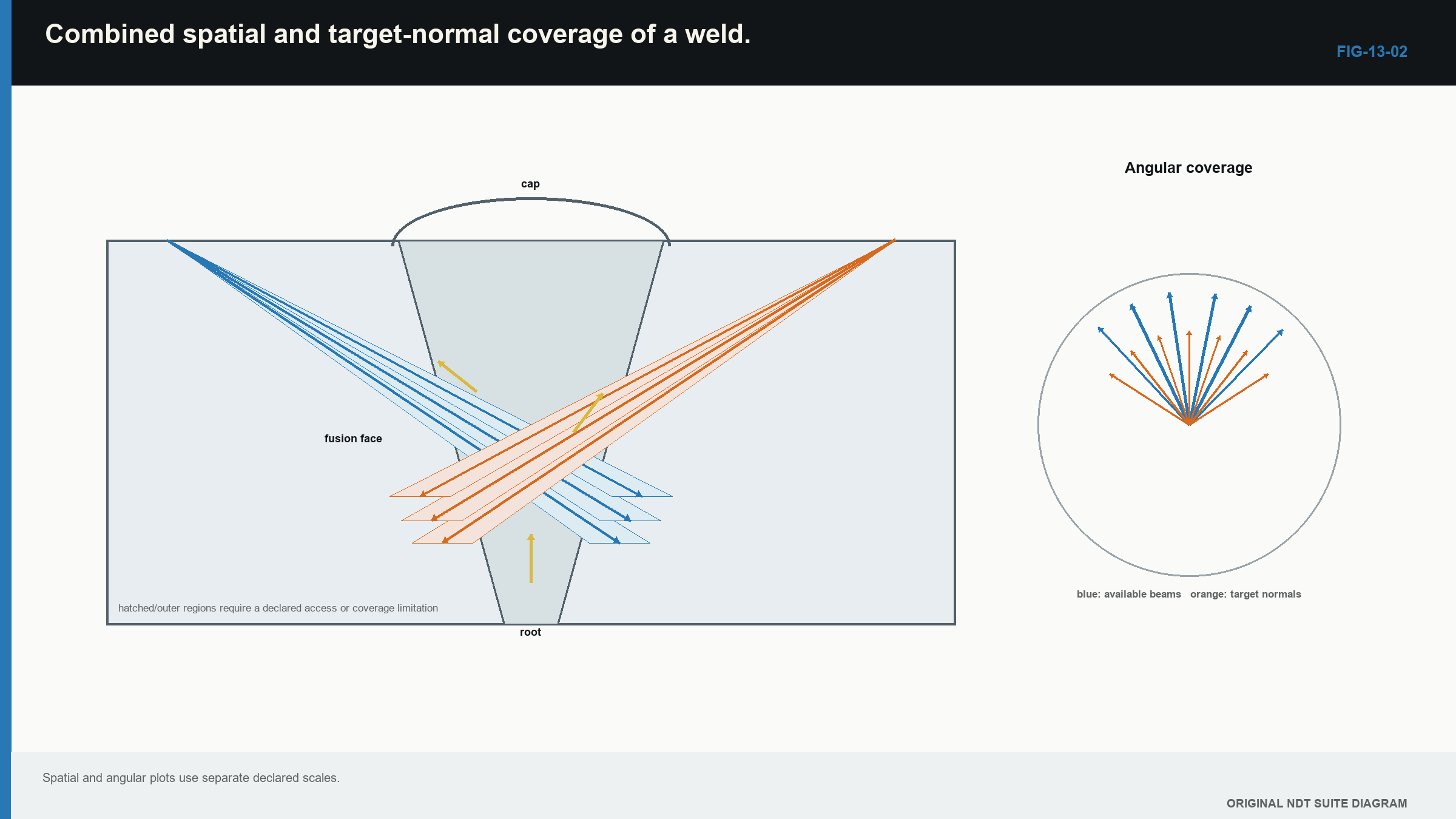
Opposite-side access can improve orientation and reduce some geometry ambiguities. It does not automatically make the two views independent if they share the same wrong thickness, angle or material model.
13.8 Connect encoded data rate to scan speed
Along-scan spacing depends on speed and the rate at which complete records are stored. The practical relationship is:
required complete-record rate = scan speed divided by allowed position interval
| Worked example · Check whether the record rate supports scan spacing WE-13-03 Given: Planned scan speed is 120 mm/s. Maximum allowed along-scan interval is 0.4 mm. Find: Minimum complete-record rate. Steps: Divide speed by interval. record rate = 120 mm/s / 0.4 mm = 300 records/s Answer: At least 300 complete acquisitions per second are required. What it means in practice: A multichannel or array system may need many pulse events for one complete record. The available rate needs operating margin. Common mistake: Using pulser PRF or display refresh as if either were automatically the complete-record rate. |
|---|
Overspeed creates gaps. Smooth scanner motion does not prove complete storage. Check actual encoded positions, record counters and any dropped-data indication.
13.9 Identify shadows and inaccessible regions
Geometry can block probe placement or redirect sound. A lamination below the scanning surface can shadow part of a weld. A strong internal reflector can mask a weaker response behind it. Coarse material can reduce the usable field below the required signal-to-noise.
An alternative angle, surface or mode may recover the region. That recovery must be shown. Two partial views are not automatically one complete examination.
For the recurring plate case, a lamination survey before angle-beam weld scanning can reveal a blocked entry area. For the weld case, a large cap or attachment should be placed on the coverage drawing. For the corrosion case, rough wall may limit the depth region where a back wall can be identified.
The limitation is part of the technical result. A report form with no convenient box does not make the unexamined area disappear.
13.10 Challenge the plan with real evidence
The final plan should be challenged at the weakest positions. Known reflectors or representative targets can check shallow, deep, edge and unfavourable orientation regions. Actual scan motion can check encoder pitch and access.
Coverage evidence has four parts:
- Geometry shows that a usable path can reach the region.
- Field evidence shows enough response around the central ray.
- Scan sampling shows that the field is placed often enough.
- A representative target shows that the required interaction can be observed.
The Level 2 conclusion should state the supported region and important conditions. Formal uncertainty expansion and three-dimensional coordinate transforms are developed later. At this stage, the reader must recognise that angle, index, thickness and position variation consume coverage margin.
General UT standards describe principles but do not provide one universal scan extent for every application. The relevant product, procedure and contract supply the job requirements. [R041] The practical geometry and coverage principles here retain the international UT training foundation. [R001]
In plain words
- Draw the as-built component and coordinate datum before placing the probe.
- A central ray shows a possible path, not complete sensitivity.
- Planar target direction matters as much as target position.
- Probe footprint and access can remove a theoretically useful position.
- Scan-line spacing should be related to a declared beam width at the target depth.
- Encoded scan speed must suit the rate of complete stored records.
- Shadows, inaccessible regions and conditional coverage belong in the result.
Key terms
- Datum: a repeatable coordinate reference.
- Skew: beam rotation in the scanning-surface plane.
- Fusion face: joint-preparation face intended to fuse.
- Coverage: supported examination of a defined region and target class.
- Occlusion: blockage of a path by geometry or another boundary.
- Raster scan: parallel tracks used to sample an area.
- Overspeed: movement that produces excessive spacing or missing data.
Key relationships
- x_probe = x_target - z_target tan(theta) places a first-leg central ray at a target.
- overlap = beam width - scan spacing gives nominal contour overlap.
- record rate = scan speed/position interval links motion to encoded sampling.
Common mix-ups
- A ray crossing the weld is not proof of volume coverage.
- Spatial coverage is not target-orientation coverage.
- Probe index is not necessarily the front of the wedge or encoder origin.
- PRF is not automatically the complete-record rate.
- Interpolation does not repair missing encoded positions.
Bridge to Chapter 14
Chapter 13 assumed the material carried the planned beam in a reasonably predictable way. Chapter 14 explains why two components with the same drawing can behave very differently after casting, rolling, forging, welding, service or repair.
Sources and further study
- [R001]
- [R041]
Study and revision only. This is not an approved inspection procedure, acceptance criterion or qualification.