What Steering and Focusing Change on the Screen

Why this matters

A setup can draw a perfect centreline while the real beam remains wide, weak or split into unwanted directions. Level 2 work does not require a full field derivation, but it does require a practical model of what the screen may show. Changing angle, focus, aperture or frequency changes more than the ray. This chapter separates the nominal centreline from the useful beam region, the focus from the surrounding field, and the main response from side and grating responses. It begins with visible effects and adds only the timing calculation needed to connect those effects to the array.

What you already need

• Selected elements form a physical aperture.
• Element contributions combine according to their timing.
• A focal law can steer and focus one beam condition.
• Element directivity limits the useful angular contribution.
• An S-scan arranges responses from several laws.

What you will learn

• Predict practical screen changes when angle, focus, aperture or frequency changes.
• Separate beam centreline, beam width and focus region.
• Distinguish near-surface resolution from acoustic near-field behaviour.
• Recognise main-lobe, side-lobe and grating-lobe responses.
• Explain why a smaller law step does not create a narrower physical beam.
• Calculate the adjacent-element delay for a simple steering example.

Words you will meet

• Main lobe: the intended strongest region of the combined field.
• Beam width: the lateral width measured using a stated field or response rule.
• Focal region: the finite region around the intended focus where concentration remains useful.
• Side lobe: a weaker off-axis region produced by a finite aperture.
• Grating lobe: an unwanted strong direction caused by regular spatial sampling and phasing.
• Axial resolution: ability to separate responses along the beam or time direction.
• Lateral resolution: ability to separate responses across the beam.

30.1 Start with four setup changes

Keep one reference reflector and probe position fixed. Change one setup property at a time and watch the underlying A-scans as well as the sector view.

Change the steering angle. The nominal centreline rotates and meets different parts of the component. Echo time and corrected position can change. Response amplitude may rise or fall because reflector orientation, wedge transmission, element directivity and path length change. The same reflector can be strong over a few laws and weak elsewhere.

Change the focal depth. Sensitivity and lateral separation may improve near the selected region and worsen away from it. The response can look narrower near the intended focus, but focus is finite and depends on the actual field. A deeper focus is not automatically sharper.

Change the aperture. A larger selected aperture can increase sensitivity and narrow the main beam under suitable conditions. It can also reduce steering freedom, change near-field structure, enlarge the contact footprint and leave fewer positions for electronic stepping.

Change frequency. Higher frequency means shorter wavelength in the same mode and material. It may support improved resolution, but attenuation and scattering usually increase. Pulse length and bandwidth matter as well. A nominal frequency change can alter noise and lobe behaviour, not only spot size.

These are practical tendencies, not guarantees. Wedge, material, target and system response can reverse the simple expectation. Compare changes using a suitable target over the actual path range.

30.2 A centreline is not a beam boundary

Ray plots usually draw one line for each focal law. That line marks a nominal travel direction or calculated path. The ultrasonic field occupies a region around it. Pressure and receive sensitivity vary across that region, and the usable boundary depends on the measurement rule.

Beam width might be stated at a particular amplitude drop from the peak, between responses from a reference target, or by another controlled criterion. Different rules give different widths. A colourful software envelope without a declared level is not a measurement.

The beam also changes with distance. A width measured near the focus cannot be applied automatically at the near surface, far surface or a skip leg. Steering can make the field asymmetric. Refraction and material structure can alter it further.

This distinction explains why dense central rays do not prove coverage. Two neighbouring laws may have overlapping fields, or a gap may remain between their useful regions. A small angular increment changes the sampling of nominal directions. It does not make each physical beam narrower.

30.3 Resolution has a direction

Axial resolution describes the ability to separate two responses that lie one behind the other along the sound path. It depends strongly on pulse duration and processing. If the first pulse is still ringing when the second echo arrives, the responses can merge.

Lateral resolution describes the ability to separate two reflectors across the beam in the active plane. It depends on beam width at their location and on how the response is sampled as aperture or probe position changes.

Angular resolution describes the ability to distinguish responses by direction across a law sequence. It depends on the physical field and target response, not only the programmed angular step. A reflector can appear on several laws because neighbouring beams overlap.

Near-surface resolution is the ability to separate an early component response from the entry, wedge or probe-related signal. It is not the same as the acoustic near field. The near field describes interference structure close to an aperture. The two can influence the same region, but one is a response-separation problem and the other is a field region.

When a screen feature looks merged, identify the direction of the separation problem. Changing scan increment cannot shorten a long pulse. Changing bandwidth may help axial separation but may not narrow the lateral beam. Naming the direction prevents random setup changes.

30.4 Focus is a region, not a dot

The focal-law calculator can time elements so their contributions are predicted to arrive together near a selected point or depth. The strongest concentration occurs over a finite region. Away from that region, beam width and sensitivity change gradually.

The focused region is often described by a focal spot and focal zone. Their measured size depends on aperture, wavelength, steering, passive-plane behaviour and the criterion used to define the boundary. A focus entered as “30 mm” does not prove a 30 mm deep reflector will appear as a point.

Focus in the active plane does not guarantee equal focus in the passive plane. A linear array can control timing along its element row but normally has fixed elevation geometry. A response may be narrow in the sector plane and broader across the probe width.

Fixed transmit focus is built into a focal law. Several separate focal laws can be made for different focus depths, but each adds a firing and may create transitions in sensitivity. Some systems apply receive focusing that changes with time, often called dynamic depth focusing. Its implementation and evidence must be understood before assuming that every depth has identical resolution.

At Level 2, use focus as a controlled region that must be checked with suitable targets. Part V derives approximations for near field, focal spot, focal zone and effective aperture.

30.5 The beam contains a main lobe and side structure

The main lobe is the intended region of strongest combined response. A focal-law centreline normally follows its nominal direction. Finite apertures also produce weaker regions away from the main lobe. These are side lobes.

A side-lobe response can place a real geometric or material reflector at a misleading apparent beam direction. The reflector is real, but the interpretation based on the main-lobe centreline can be false. A repeatable response is therefore not automatically a main-beam response.

A grating lobe is a stronger unwanted direction associated with regular element spacing and phasing. It is more likely when pitch is large relative to wavelength and when steering demand increases. The exact onset depends on wedge, interface, element directivity and the selected model. The practical symptom can be a duplicate or displaced response that changes with law angle or frequency.

Side lobes are not the same as grating lobes. Side lobes occur with any finite aperture. Grating lobes arise from spatial repetition in the array and can become much more prominent. Both can produce off-axis sensitivity that a single centreline does not show.

Other misleading responses can come from internal wedge echoes, mode conversion, repeated surface paths, electronic cross-talk, poor element connections and geometric reflections. Diagnosis should compare time, position, law dependence, probe movement and known geometry before assigning a lobe label.

30.6 Pitch, width and wavelength influence lobes

Element pitch sets the regular centre spacing of the array. Wavelength is wave speed divided by frequency for the stated mode and material. Their ratio affects how the contributions can reinforce in unintended directions.

Element width also matters because directivity can suppress some off-axis contributions. Pitch and width are therefore related but not interchangeable. Two arrays can have the same pitch and different kerf or element width, giving different element directivity and electrical behaviour.

Steering farther from the natural direction increases the timing slope across the aperture. At the same time, the projected aperture and interface transmission may change. A law set that behaves well near its centre can become weak or lobe-prone at its edges.

Do not infer a universal acceptable pitch ratio from this chapter. The wedge and refracted component field must be considered, and the selected probe-wedge-law combination must be characterised over its claimed range. Part V develops the detailed limits and broadband behaviour.

30.7 Connect steering to adjacent-element delay

Electronic steering begins with a simple physical requirement: contributions from neighbouring elements must be started at different times so they line up along the intended direction. For a uniform row in one material, a basic adjacent delay is related to pitch, steering angle and sound speed.

In words:

adjacent delay = sideways path difference between element centres divided by wave speed

The sideways path difference for a direction at angle theta from the array normal is p sin(theta).

This relationship is not the complete law for a wedge-coupled inspection. A real focal-law calculation includes element positions, wedge paths, refraction, selected focus and receive timing. The simple form shows why greater pitch or angle needs a larger adjacent delay and why higher speed needs a smaller delay for the same geometry.

30.8 Read the screen without over-reading it

The following figure links delay patterns to main and unwanted field regions. Use it to name the parts, not to measure them. [R014] [R016]

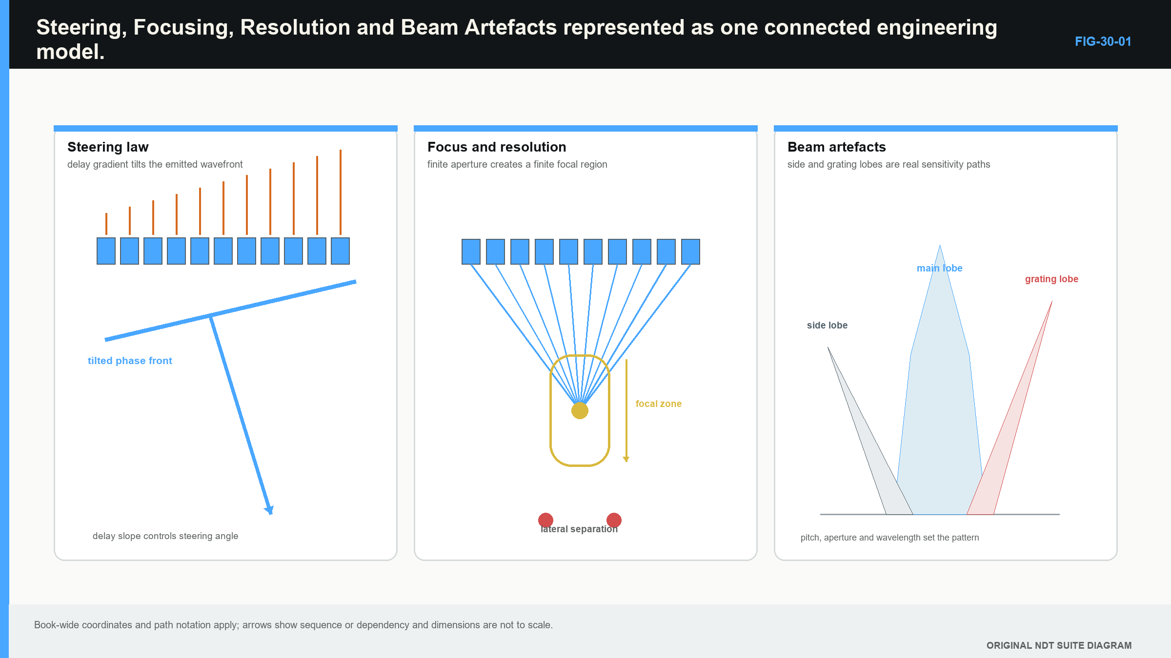
When a feature changes after a setup adjustment, describe the change before explaining it. State whether echo time, peak amplitude, width across laws, width along scan, noise or corrected position changed. Then identify which physical effect the adjustment could influence.

For example, a response that remains at the same A-scan time but appears on a different law after an angle change may reflect remapping or a different beam interaction. A response duplicated at a consistent offset over several probe positions may suggest an off-axis or geometric path. A broad response near the selected focus may indicate that target orientation or passive-plane width dominates the display.

Use reference targets that challenge the required depth and angle range. A strong target on the centre law does not establish performance at the sector edges. A target at the focus does not prove near- and far-surface resolution. One target also cannot distinguish every artefact mechanism.

Detailed apodisation, bandwidth measurement, quality factor, broadband lobe prediction and point-spread-function analysis are moved to Part V. They matter, but Level 2 first needs a stable link between a setting, its physical effect and the observed response.

Four practical screen comparisons

The peak becomes narrower across scan position. First confirm that the acquisition increment did not change. If spacing is unchanged and the reflector is comparable, a larger or better-focused aperture may have narrowed the active-plane response near that depth. The result does not prove a smaller physical reflector.

The peak becomes shorter in time. Check whether frequency response, damping, filtering or rectification changed. A shorter pulse can improve axial separation, but a display envelope can also look shorter because of threshold or smoothing. Return to the same RF waveform representation before drawing a resolution conclusion.

A duplicate feature appears at a law-dependent offset. Compare its time relationship with a strong known reflector. Observe whether it changes when steering range, aperture or frequency changes. That pattern can support an off-axis, repeated-path or mode-converted explanation. It does not identify the mechanism without the corresponding path check.

The sector edges require much more correction gain. Review raw response before equalisation. Weak edge laws can reflect directivity, wedge transmission, aperture projection or target orientation. Raising them to the same colour level may also raise noise and unwanted responses. The usable sector may need to be narrower than the programmed sector.

For every comparison, change one main variable while reproducing the target, probe position and display basis. Simultaneous changes to angle, aperture, focus, filter and gain produce a different image but little diagnostic knowledge. The study skill is to connect one controlled change to one observed effect and one remaining uncertainty.

Use the same comparison at several depths. A focus adjustment may sharpen a reference response near its selected region while broadening or weakening it elsewhere. An aperture that performs well at mid-wall may behave differently near the entry surface or after a reflection. Sector-edge laws may also lose useful response more rapidly with path.

Keep a simple observation sheet with setup change, unchanged controls, target, path, A-scan effect, sector effect and remaining explanation. This discourages conclusions based only on one saved image. It also reveals trade-offs: a change can improve one response while reducing another part of the required volume.

When two settings produce similar bright images, prefer the one whose physical behaviour and operating margin are easier to demonstrate. The most attractive picture is not automatically the most stable technique. Repeatability across position, path and realistic coupling is more useful than a single narrow peak obtained under perfect alignment.

These comparisons prepare the reader for Level 3 field maps. They do not require pressure calculations, but they establish the experimental discipline those calculations must eventually match.

Keep centreline, width and response extent in separate columns during the trial. The centreline comes from the law model. Width comes from a stated measurement criterion. Response extent comes from the chosen target and scan. Agreement can support the model, while disagreement shows which assumption needs investigation.

Apply the same separation to focus. Record entered focus, target depth and observed width or amplitude. A narrow response near the entered value supports one bounded observation. It does not establish the complete focal-zone shape above and below it.

Repeat a selected observation after removing and replacing the probe. Large changes can expose contact or positioning sensitivity that a stationary comparison hides. This matters because production scanning repeatedly changes local couplant thickness and pressure. A field behaviour that exists only under one carefully held position has limited practical value.

In plain words

• A ray is a nominal centreline, not the edge of the sound field.
• Beam width depends on distance and on the rule used to measure it.
• Axial, lateral and angular resolution describe different separation problems.
• Near-surface resolution is not the same as acoustic near field.
• A focus occupies a finite region and can differ between active and passive planes.
• Side lobes and grating lobes can create responses away from the intended centreline.
• Smaller angular steps add more sampled directions but do not narrow the physical beam.
• Steering delays are small timing differences whose value depends on geometry and wave speed.

Key terms

Centreline; beam width; axial resolution; lateral resolution; angular resolution; focus; focal region; main lobe; side lobe; grating lobe.

Key relationships

• aperture, frequency, steering and path -> beam width and focal behaviour;
• shorter pulse -> potentially better axial separation;
• narrower main beam -> potentially better lateral separation;
• pitch relative to wavelength + steering demand -> grating-lobe risk;
• adjacent path difference divided by speed -> adjacent timing delay;
• programmed law step != physical beam width.

Common mix-ups

• Near-surface resolution is not near field.
• The focus value is not the size of the focal spot.
• Side lobes and grating lobes are not identical.
• Pitch is centre spacing; element width is not automatically equal to pitch.
• A dense ray plot is not a coverage proof.

Bridge to Chapter 31

Chapter 31 turns one focal law into purposeful sequences. It separates physical probe movement, electronic aperture movement, angle sweeps and focus sweeps, then counts the laws that the instrument must actually execute.

Sources and further study

• [R014]
• [R016]