Choosing Modes, Views and Acoustic Paths

Why this matters

FMC stores waveforms, not labels for the routes that created each echo. Reconstruction software must assign a transmit path and a receive path before it can calculate a pixel. A direct shear view, a backwall-reflected view and a mode-converted view can all produce persuasive images from the same source data. The Level 2 task is to draw each route, name every mode and boundary, and retain only the small set that has a physical purpose and demonstrated response.

What you already need

• The Chapter 49 two-leg travel-time picture.
• Longitudinal and shear-wave speed differences.
• PAUT first-leg, second-leg, skip and reflector-orientation knowledge.
• Basic reflection, refraction and mode-conversion awareness.
• The difference between a ray reaching a region and a target returning useful energy.

What you will learn

• Define a TFM view through its transmit and receive routes.
• Read and write simple neutral path labels.
• Compare direct longitudinal, direct shear, reflected and mode-converted paths.
• Calculate a piecewise path time with more than one mode.
• Relate view choice to specular, corner and diffracted responses.
• Expose geometry responses and path ambiguity before interpretation.

Words you will meet

• View: an image formed with one declared transmit path and receive path.
• Direct path: route without an internal component-boundary reflection.
• Reflected path: route that deliberately uses a known component boundary.
• Mode-converted path: route containing more than one wave mode.
• Specular response: mirror-like return favoured by a particular surface orientation.
• Diffraction: weaker energy spread from an edge or tip over a wider angle range.
• Path degeneracy: different physical routes having similar travel times or image solutions.

50.1 Carry PAUT path thinking into one TFM view

In PAUT, a scan plan links probe position, angle, mode and skip route to a target region; a view extends that familiar reasoning across both sides of an FMC pair. It declares how sound travels from the transmitting element to a candidate interaction and how it returns to the receiving element. The source traces do not decide that route; the reconstruction chooses it. That choice fixes the predicted time, image location and target orientations likely to return energy. A view name is therefore useful only when it can be translated into a complete physical drawing.

Open multi-view research and guidance describe reconstruction through explicit transmit and receive path families and warn that path selection governs both useful coverage and artefact formation. [R018] [R019] [R047] Start with a small canonical set. Use direct longitudinal, direct shear, one backwall-reflected route and one deliberately supported mode conversion. Additional views are added only when they close a named orientation or access gap.

50.2 Direct longitudinal and direct shear views

A direct L-L view uses longitudinal-wave propagation on the transmit side and longitudinal-wave propagation on the receive side inside the component. It can be useful for normal or near-normal access, volumetric reflectors and surfaces oriented to return longitudinal energy. A direct T-T view uses transverse, or shear, propagation on both sides; an angle-beam wedge normally supplies a longitudinal wedge leg before refraction into the specimen shear mode. The label describes the specimen legs; the complete drawing still shows the wedge and interface.

Direct means that no internal component-boundary reflection has been inserted between the array and the candidate point; it does not mean that the real route is simple. Curved surfaces can create element-specific entry points; large departure angles may exceed useful element directivity. A smooth vertical planar reflector may return specular energy away from the aperture even when the ray reaches it. The following figure adds views one at a time. Notice that every panel includes separate transmit and receive sides.

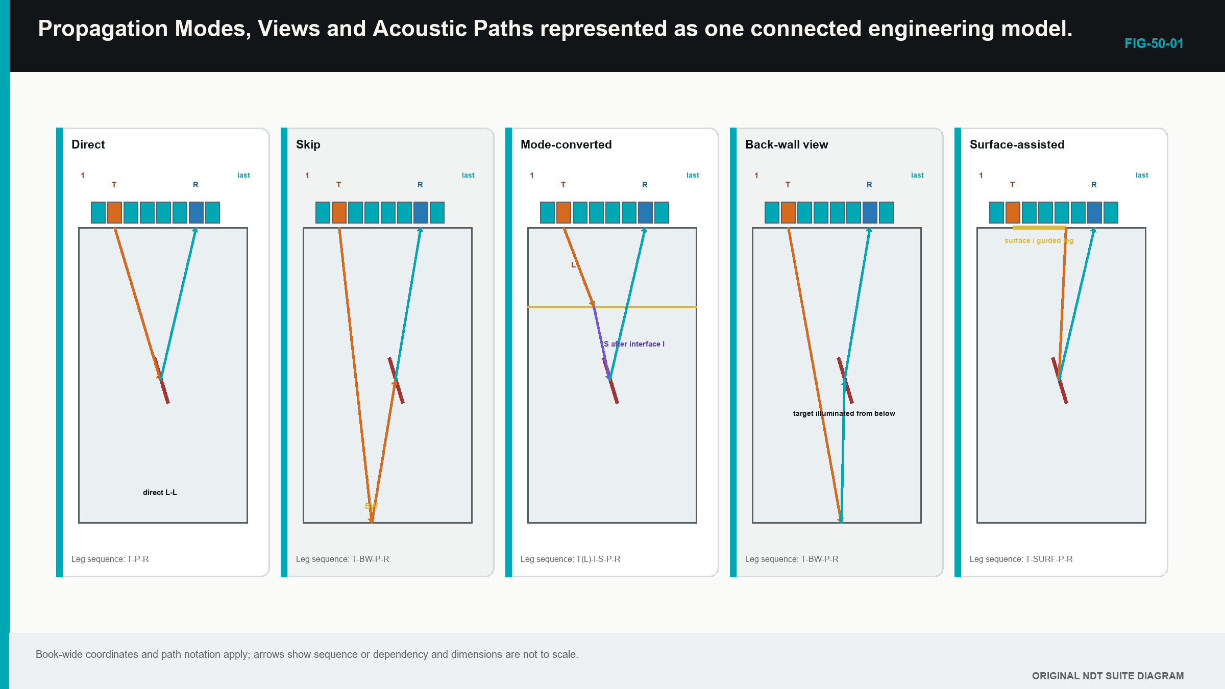
The direct panels are the reference. A more complicated view should explain what the direct view cannot reach or what target orientation it cannot return.

50.3 Add one reflected route

A reflected path deliberately uses a known boundary, often the backwall. Conventional angle-beam work already uses first and second legs. Matrix imaging can place a reflection on only the transmit side, only the receive side or both.

For a TT-T example, the transmit route has two shear legs separated by a backwall reflection, while the receive route returns directly in shear. T-TT reverses those sides. A TT-TT route uses a declared reflection on both sides.

The doubled letter is only a compact label; the drawing must still identify the reflecting surface, reflection point, component thickness, pixel position and active aperture. A term such as half skip can become ambiguous when the two sides have different leg counts, so the diagram remains the primary definition.

Each reflection adds risk; the boundary may be rough, curved, corroded or clad. The calculated point can fall outside the real surface. Path length and attenuation increase. Geometry responses can share similar times. A ray that reflects neatly on a nominal drawing does not prove useful energy follows that route in the component.

Reflected and tandem-like views can improve access to steep planar targets or their tips; their performance is established with representative targets at difficult locations, not inferred from a strong central backwall.

50.4 Add one mode conversion

At a boundary or reflector, incident energy can produce a different wave mode; a selected view can model that conversion. For example, a transmit route can include a longitudinal leg followed by a shear leg, while the receive side remains shear.

The route uses the correct speed for each leg. Treating a mixed path with one average velocity changes the predicted time and phase alignment; the interface angle, material pair and polarisation also govern whether enough energy converts to be useful.

Mode conversion is not free coverage; a valid geometric route can have a very small conversion coefficient or direct energy away from the aperture. Unmodelled conversion can also create a false feature. A real L-T arrival reconstructed as L-L may partly align at another coordinate.

The Level 2 learner records the conversion, checks that the implementation supports it and compares it with a known target. Formal transmission coefficients and solver limits belong in Chapters 57 and 66.

50.5 Use neutral path notation gradually

The hyphen separates the transmitter-to-pixel sequence from the pixel-to-receiver sequence. Letters on each side list specimen modes and leg count in order. The first working set is:

• L-L for direct longitudinal transmit and receive;
• T-T for direct shear transmit and receive;
• TT-T for a reflected two-leg shear transmit route and direct shear receive;
• T-TT for the reciprocal ordering; and
• LT-T for a declared longitudinal-to-shear transmit sequence and direct shear receive.

The notation is deliberately vendor-neutral. A product can use names such as wave set, self-tandem, intermode or a branded combined view. The controlled implementation profile translates that label into the actual path. A software menu entry is not the physical definition.

Transmit and receive order matters. Reversed routes may look similar under reciprocal conditions, but different electronics, pair masks, sub-apertures, transmission directions or acquisition timing can make their displays differ. Missing reciprocal data must not be invented.

50.6 Calculate time leg by leg

The physical relationship is simple once every leg is drawn. Divide each leg length by the speed of its declared mode, then add the times.

The units check is metres divided by metres per second for each leg, producing seconds. A reflected route normally has a longer time than a direct route to a similar region. A mixed-mode route can also be slow because the shear segment uses the lower speed.

50.7 Match the view to reflector behaviour

A small pore or compact volumetric target can scatter over a useful angular range. A direct view may therefore show it across many pair angles. A side-drilled hole is an extended cylinder rather than an ideal point, so its response still depends on orientation and mode.

A smooth planar surface behaves more like a mirror. Strong specular response occurs only when the incident and receive geometry favour a return to the aperture. A direct view can cross the plane without seeing its face strongly. A reflected or tandem-like view may provide a more favourable return.

A crack tip or notch end can produce diffraction over a wider angular range, usually with weaker energy than a favourable face or corner. Complementary views can seek upper and lower tip evidence. A corner formed between a planar reflector and a component surface can create a strong corner-trap response.

Different views can therefore emphasise different parts of one physical feature. A face in amplitude TFM and two compact tips in PCI are not automatically contradictory. They require common coordinates, plausible paths and demonstrated target behaviour.

50.8 Account for aperture, directivity and shadow

A drawn ray establishes geometric possibility. Sensitivity also depends on whether the selected elements transmit and receive effectively along the route. Finite element directivity reduces useful contribution at large angles. Wedge transmission, attenuation and path length further change the response.

At one ROI edge, only a central portion of the array may provide useful pairs. At another location, a boundary or previous interface can shadow the target. A point with few contributing pairs can be normalised to look as bright as a fully supported point unless the processing exposes support.

A useful coverage record identifies element contributions, reflection points, directivity limits, shadow zones and the region where one view hands over to another. The model guides target placement. Representative reflectors then establish actual detection, position and separation behaviour through the intended material.

Adding every available view does not fix a coverage gap. More views increase processing and the number of benign routes that can align. Each retained view needs one stated purpose.

50.9 Recognise geometry and path degeneracy

Backwalls, sidewalls, counterbores, weld roots, caps, cladding boundaries and wedge echoes are real acoustic reflectors. Reconstruction software does not know whether their energy is relevant. If the timing fits the selected path to a pixel, the event can be displayed.

Path degeneracy occurs when different physical routes produce similar times or locations. A boundary echo in one mode can resemble a target echo under another. A direct event can be reconstructed with a skip model, or a mode conversion can appear under a same-mode label. The image may remain coherent because real energy exists; the interpretation is still wrong.

Predict benign geometry before examining unknown indications. Compare response movement as the probe advances. Inspect source A-scans and aperture support. Reconstruct a competing plausible path on a working copy. Use views whose physics differs meaningfully, rather than counting several near-identical displays as independent confirmation.

If two views place the same claimed feature at incompatible coordinates, investigate velocity, thickness, surface, time origin and path. A clean merged display can hide that disagreement, so retain the individual views.

50.10 Select a small justified view set

Begin with the component drawing, access, materials and target orientations. Draw direct L and T candidates. Add one reflected or converted route only when it closes a named gap. Label transmit and receive sides, modes, boundaries and velocities. Confirm that interface and reflection points lie inside real surfaces.

Next consider directivity, aperture support, path length, attenuation and expected scattering direction. Predict backwall, root and sidewall responses. Select reference targets that challenge the view near its shallow, deep and lateral limits.

Reject a geometrically impossible route even if a reconstruction looks attractive. Reject a physically possible route that has no useful target purpose or demonstrated sensitivity. Freeze the remaining set with its ROI, aperture and implementation identity.

A completed planning case for a butt weld might retain direct T-T for volumetric and favourably oriented response, TT-T for a steep planar face, T-TT for reciprocal comparison and one supported converted view for a specific corner. Two other candidates are documented as rejected because one reflection point falls outside the backwall and one arrives within time support but lacks target sensitivity.

50.11 Level boundary and path-validity gates

At Level 2, a path is acceptable for supervised use only when its legs, modes, surfaces, times, aperture and target purpose can be explained under the controlled technique. The learner can calculate piecewise times and recognise uncertainty. Formal root finding, curved-interface solvers, anisotropic slowness and path-identifiability analysis belong later.

Chapter 57 develops path solvers and model error. Chapter 62 develops forensic checks for ambiguous modes and geometry responses. Chapters 65, 66 and 72 add the engineering physics and imaging detail.

A Level 3 validity gate can test interface intersection, incidence range, mode existence, component boundaries and trace-time support for every pixel. It also compares paths on targets where competing solutions separate. If the validation set never distinguishes two routes, the technique cannot claim that the image distinguishes them. [R018] [R019] [R047]

In plain words

• A view is defined by both its transmit route and its receive route.
• Direct L-L and T-T views should be understood before reflected or converted paths are added.
• Every reflected surface and mode conversion must appear in the drawing and time calculation.
• A ray reaching the target region does not prove useful transmitted and received energy.
• Smooth faces, corners, tips and volumetric targets return energy differently.
• Geometry and valid but unintended paths can produce coherent image features.
• A small justified view set is stronger than a gallery of unexplained reconstructions.
• Vendor labels must translate into explicit physical paths.

Key terms

• View: image calculated for one declared transmit and receive path family.
• Direct path: route without an internal boundary reflection.
• Reflected path: route that intentionally includes a known boundary.
• Mode-converted path: route in which the wave mode changes.
• Specular response: orientation-sensitive mirror-like return.
• Diffraction: energy spread from an edge or tip.
• Path degeneracy: competing routes with similar time or image solutions.

Key relationships

• view = transmit route + receive route: both sides define the image assumption.
• t_P = sum(d_k/c_k): calculate time one declared leg and mode at a time.
• geometric access + useful aperture + target scattering: all three support a practical view.
• more views != more proof: each additional view also introduces alternative paths and artefacts.

Common mix-ups

• Direct does not mean interface-free when a wedge is present.
• A path label without a surface and leg diagram is incomplete.
• Reciprocity is a diagnostic expectation, not guaranteed identical displayed views.
• Matching travel time does not establish matching physical cause.
• A strong geometry response is coherent evidence but not necessarily a relevant discontinuity.

Bridge to Chapter 51

Chapter 50 has selected the physical routes. Chapter 51 controls how those routes are calculated and displayed across the ROI. It begins with one unchanged dataset shown at different pixel spacing, aperture, bandwidth and normalisation so the effect is seen before the parameter is named.

Sources and further study

• [R018]
• [R019]
• [R047]